18 Image classification, take two: Improving performance

In the last two chapters, we saw how changes to data input, network architecture, and training modalities can result in improved results, “improvement” having two principal denotations: better generalization to the test set, and faster training progress.

Now, we’ll apply a few of those techniques to the image classification task we started our journey into real-world deep learning with: Tiny Imagenet. In terms of counteracting overfitting, we’ll introduce data augmentation, dropout layers, and early stopping. To speed up training, we make use of the learning rate finder, add batchnorm layers, and integrate a pre-trained network. We won’t add-and-remove these techniques one at a time, that is, we won’t assess their effects in isolation. While this is something you might want to do yourself, here we want to avoid the impression that there is some fixed ranking – this is best, that is second … – , independently of dataset and task.

Instead, what we do is:

Always use data augmentation. There is hardly ever a case where you’d not want to use it – unless, of course, you are already using a different data augmentation technique.
Always run with early stopping enabled. This will not just prevent overfitting, but also, save time.
Always make use of the learning rate finder, together with a one-cycle learning rate schedule.
For our first setup, we take the convnet from three chapters ago, and add dropout layers.
In scenario number two, we replace dropout by batch normalization. (Everything else stays the same.)
Third, we replace the model completely, by one chaining a pre-trained feature classifier (ResNet) and a small sequential model.

18.1 Data input (common for all)

All three runs use the same data input pipeline. Compared with our first go at telling apart the two hundred classes in Tiny Imagenet, two things are new.

First, we now apply data augmentation to the training set: rotations and translations, to be precise.

Second, input tensors are normalized, channel-wise, to a set of given means and standard deviations. This really is required for the third run (using ResNet) only; we just do to our images what was done in training ResNet. (The same goes for most of the pre-trained models trained on ImageNet.) There really is no problem, though, in doing the same for runs one and two; so normalization is part of the common pre-processing pipeline.

library(torch)
library(torchvision)
library(torchdatasets)
library(luz)

set.seed(777)
torch_manual_seed(777)

dir <- "~/.torch-datasets"

train_ds <- tiny_imagenet_dataset(
  dir,
  download = TRUE,
  transform = . %>%
    transform_to_tensor() %>%
    transform_random_affine(
      degrees = c(-30, 30), translate = c(0.2, 0.2)
    ) %>%
    transform_normalize(
      mean = c(0.485, 0.456, 0.406),
      std = c(0.229, 0.224, 0.225)
    )
)

valid_ds <- tiny_imagenet_dataset(
  dir,
  split = "val",
  transform = function(x) {
    x %>%
      transform_to_tensor() %>%
      transform_normalize(
        mean = c(0.485, 0.456, 0.406),
        std = c(0.229, 0.224, 0.225))
  }
)

train_dl <- dataloader(
  train_ds,
  batch_size = 128,
  shuffle = TRUE
)
valid_dl <- dataloader(valid_ds, batch_size = 128)

Next, we compare three different configurations.

18.2 Run 1: Dropout

In run one, we take the convnet we were using, and add dropout layers.

convnet <- nn_module(
  "convnet",
  initialize = function() {
    self$features <- nn_sequential(
      nn_conv2d(3, 64, kernel_size = 3, padding = 1),
      nn_relu(),
      nn_max_pool2d(kernel_size = 2),
      nn_dropout2d(p = 0.05),
      nn_conv2d(64, 128, kernel_size = 3, padding = 1),
      nn_relu(),
      nn_max_pool2d(kernel_size = 2),
      nn_dropout2d(p = 0.05),
      nn_conv2d(128, 256, kernel_size = 3, padding = 1),
      nn_relu(),
      nn_max_pool2d(kernel_size = 2),
      nn_dropout2d(p = 0.05),
      nn_conv2d(256, 512, kernel_size = 3, padding = 1),
      nn_relu(),
      nn_max_pool2d(kernel_size = 2),
      nn_dropout2d(p = 0.05),
      nn_conv2d(512, 1024, kernel_size = 3, padding = 1), 
      nn_relu(),
      nn_adaptive_avg_pool2d(c(1, 1)),
      nn_dropout2d(p = 0.05),
    )
    self$classifier <- nn_sequential(
      nn_linear(1024, 1024),
      nn_relu(),
      nn_dropout(p = 0.05),
      nn_linear(1024, 1024),
      nn_relu(),
      nn_dropout(p = 0.05),
      nn_linear(1024, 200)
    )
  },
  forward = function(x) {
    x <- self$features(x)$squeeze()
    x <- self$classifier(x)
    x
  }
)

Next, we run the learning rate finder (fig. 18.1).

model <- convnet %>%
  setup(
    loss = nn_cross_entropy_loss(),
    optimizer = optim_adam,
    metrics = list(
      luz_metric_accuracy()
    )
  ) 
    
rates_and_losses <- model %>% lr_finder(train_dl)
rates_and_losses %>% plot()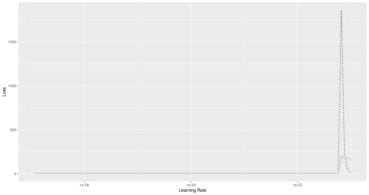

A curve that, from left to right, stays flat for a long time (until about x=0.01), then oscillates between low and higher values, and finally (at about x=0.05) starts to rise very sharply. — Figure 18.1: Learning rate finder, run on Tiny Imagenet. Convnet with dropout layers.

We already know that discerning between two hundred classes is a task that takes time; it’s thus not surprising to see a flat-ish loss curve during most of learning rate increase. We can conclude, though, that we had better not exceed a learning rate of 0.01.

As in all further configurations, we now train with the one-cycle learning rate scheduler, and early stopping enabled.

fitted <- model %>%
  fit(train_dl, epochs = 50, valid_data = valid_dl,
      callbacks = list(
        luz_callback_early_stopping(patience = 2),
        luz_callback_lr_scheduler(
          lr_one_cycle,
          max_lr = 0.01,
          epochs = 50,
          steps_per_epoch = length(train_dl),
          call_on = "on_batch_end"),
        luz_callback_model_checkpoint(path = "cpt_dropout/"),
        luz_callback_csv_logger("logs_dropout.csv")
        ),
      verbose = TRUE)

For me, training stopped after thirty-five epochs, at a validation accuracy of 0.4, and a training accuracy that was just slightly higher: 0.44.

Epoch 1/50
Train metrics: Loss: 5.116 - Acc: 0.0128                                      
Valid metrics: Loss: 4.9144 - Acc: 0.0217
Epoch 2/50
Train metrics: Loss: 4.7217 - Acc: 0.042                                      
Valid metrics: Loss: 4.4143 - Acc: 0.067
Epoch 3/50
Train metrics: Loss: 4.3681 - Acc: 0.0791                                     
Valid metrics: Loss: 4.1145 - Acc: 0.105
...
...
Epoch 33/50
Train metrics: Loss: 2.3006 - Acc: 0.4304                                     
Valid metrics: Loss: 2.5863 - Acc: 0.4025
Epoch 34/50
Train metrics: Loss: 2.2717 - Acc: 0.4365                                     
Valid metrics: Loss: 2.6377 - Acc: 0.3889
Epoch 35/50
Train metrics: Loss: 2.2456 - Acc: 0.4402                                     
Valid metrics: Loss: 2.6208 - Acc: 0.4043
Early stopping at epoch 35 of 50

Comparing with the initial approach, where after fifty epochs, we were left with accuracies of 0.22 for validation, and 0.92 for training, we see an impressive reduction in overfitting. Of course, we cannot really say anything about the respective merits of dropout and data augmentation here. If you’re curious, please go ahead and find out!

18.3 Run 2: Batch normalization

In configuration number two, dropout is replaced by batch normalization.

convnet <- nn_module(
  "convnet",
  initialize = function() {
    self$features <- nn_sequential(
      nn_conv2d(3, 64, kernel_size = 3, padding = 1),
      nn_batch_norm2d(64),
      nn_relu(),
      nn_max_pool2d(kernel_size = 2),
      nn_conv2d(64, 128, kernel_size = 3, padding = 1),
      nn_batch_norm2d(128),
      nn_relu(),
      nn_max_pool2d(kernel_size = 2),
      nn_conv2d(128, 256, kernel_size = 3, padding = 1),
      nn_batch_norm2d(256),
      nn_relu(),
      nn_max_pool2d(kernel_size = 2),
      nn_conv2d(256, 512, kernel_size = 3, padding = 1),
      nn_batch_norm2d(512),
      nn_relu(),
      nn_max_pool2d(kernel_size = 2),
      nn_conv2d(512, 1024, kernel_size = 3, padding = 1), 
      nn_batch_norm2d(1024),
      nn_relu(),
      nn_adaptive_avg_pool2d(c(1, 1)),
    )
    self$classifier <- nn_sequential(
      nn_linear(1024, 1024),
      nn_relu(),
      nn_batch_norm1d(1024),
      nn_linear(1024, 1024),
      nn_relu(),
      nn_batch_norm1d(1024),
      nn_linear(1024, 200)
    )
  },
  forward = function(x) {
    x <- self$features(x)$squeeze()
    x <- self$classifier(x)
    x
  }
)

Again, we run the learning rate finder (fig. 18.2):

model <- convnet %>%
  setup(
    loss = nn_cross_entropy_loss(),
    optimizer = optim_adam,
    metrics = list(
      luz_metric_accuracy()
    )
  ) 

rates_and_losses <- model %>% lr_finder(train_dl)
rates_and_losses %>% plot()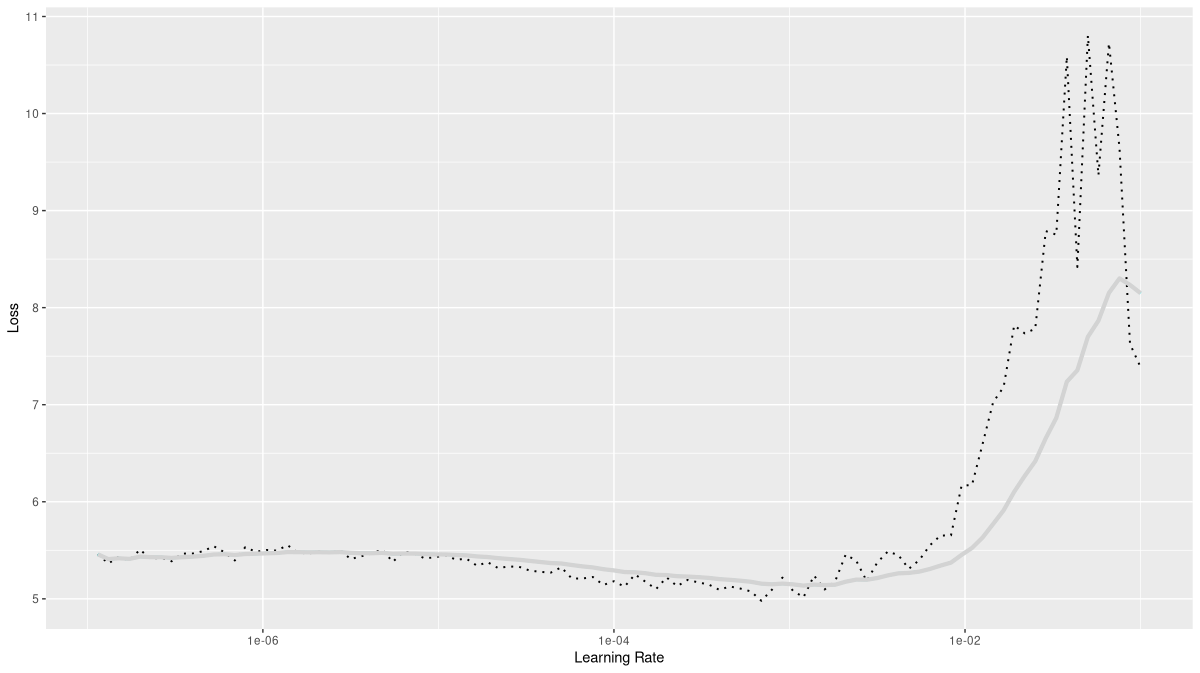

A curve that, from left to right, first descends in a smooth, accelerating curve (until about x=0.001), stays flat for a while, and then (shortly before x=0.001), begins to rise in a sharp, but still smooth, curve. — Figure 18.2: Learning rate finder, run on Tiny Imagenet. Convnet with batchnorm layers.

This looks surprisingly different! Of course, this is in part due to the scale on the loss axis; the loss does not explode as much, and thus, we get better resolution in the early and middle stages. The loss not exploding is an interesting finding in itself; the conclusion for us to draw from this plot is to be a bit more careful with the learning rate. This time, we’ll choose 0.001 for the maximum.

fitted <- model %>%
  fit(train_dl, epochs = 50, valid_data = valid_dl,
      callbacks = list(
        luz_callback_early_stopping(patience = 2),
        luz_callback_lr_scheduler(
          lr_one_cycle,
          max_lr = 0.001,
          epochs = 50,
          steps_per_epoch = length(train_dl),
          call_on = "on_batch_end"),
        luz_callback_model_checkpoint(path = "cpt_batchnorm/"),
        luz_callback_csv_logger("logs_batchnorm.csv")
        ),
      verbose = TRUE)

Compared with scenario one, I saw slightly more overfitting with batchnorm.

Epoch 1/50
Train metrics: Loss: 4.5434 - Acc: 0.0862                                     
Valid metrics: Loss: 4.0914 - Acc: 0.1332
Epoch 2/50
Train metrics: Loss: 3.9534 - Acc: 0.161                                      
Valid metrics: Loss: 3.7865 - Acc: 0.1809
Epoch 3/50
Train metrics: Loss: 3.6425 - Acc: 0.2054                                     
Valid metrics: Loss: 3.5965 - Acc: 0.2115
...
...
Epoch 19/50
Train metrics: Loss: 2.1063 - Acc: 0.4859                                     
Valid metrics: Loss: 2.621 - Acc: 0.3912
Epoch 20/50
Train metrics: Loss: 2.0514 - Acc: 0.4987                                     
Valid metrics: Loss: 2.6334 - Acc: 0.3914
Epoch 21/50
Train metrics: Loss: 1.9982 - Acc: 0.5069                                     
Valid metrics: Loss: 2.6603 - Acc: 0.3932
Early stopping at epoch 21 of 50

18.4 Run 3: Transfer learning

Finally, the setup including transfer learning. A pre-trained ResNet is used for feature extraction, and a small sequential model takes care of classification. During training, all of ResNets weights are left untouched.

convnet <- nn_module(
  initialize = function() {
    self$model <- model_resnet18(pretrained = TRUE)
    for (par in self$parameters) {
      par$requires_grad_(FALSE)
    }
    self$model$fc <- nn_sequential(
      nn_linear(self$model$fc$in_features, 1024),
      nn_relu(),
      nn_linear(1024, 1024),
      nn_relu(),
      nn_linear(1024, 200)
    )
  },
  forward = function(x) {
    self$model(x)
  }
)

As always, we run the learning rate finder (fig. 18.3).

model <- convnet %>%
  setup(
    loss = nn_cross_entropy_loss(),
    optimizer = optim_adam,
    metrics = list(
      luz_metric_accuracy()
    )
  ) 

rates_and_losses <- model %>% lr_finder(train_dl)
rates_and_losses %>% plot()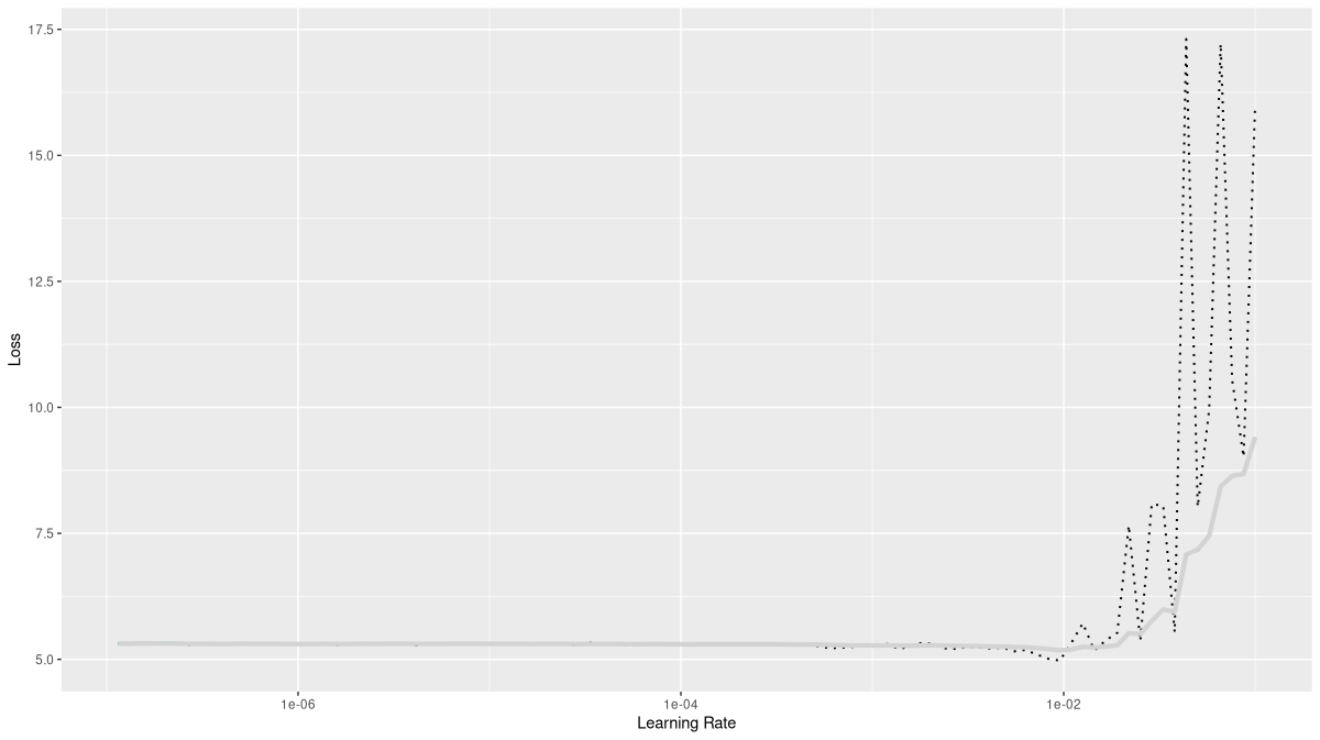

A curve that, from left to right, first stays flat (until about x=0.01), then begins to rise very sharply, while at the same time showing high variability. — Figure 18.3: Learning rate finder, run on Tiny Imagenet. Convnet with transfer learning (ResNet).

A maximal rate of 0.01 looks like it could be on the edge, but I decided to give it a try.

fitted <- model %>%
  fit(train_dl, epochs = 50, valid_data = valid_dl,
      callbacks = list(
        luz_callback_early_stopping(patience = 2),
        luz_callback_lr_scheduler(
          lr_one_cycle,
          max_lr = 0.01,
          epochs = 50,
          steps_per_epoch = length(train_dl),
          call_on = "on_batch_end"),
        luz_callback_model_checkpoint(path = "cpt_resnet/"),
        luz_callback_csv_logger("logs_resnet.csv")
        ),
      verbose = TRUE)

For me, this configuration resulted in early stopping after nine epochs already, and yielded the best results by far: Final accuracy on the validation set was 0.48. Interestingly, in this setup, accuracy ended up worse for training than for validation.

Epoch 1/50
Train metrics: Loss: 3.4036 - Acc: 0.2322                                     
Valid metrics: Loss: 2.5491 - Acc: 0.3884
Epoch 2/50
Train metrics: Loss: 2.7911 - Acc: 0.3436                                     
Valid metrics: Loss: 2.417 - Acc: 0.4233
Epoch 3/50
Train metrics: Loss: 2.6423 - Acc: 0.3726                                     
Valid metrics: Loss: 2.3492 - Acc: 0.4431
...
...
Valid metrics: Loss: 2.1822 - Acc: 0.4868
Epoch 7/50
Train metrics: Loss: 2.4031 - Acc: 0.4198                                     
Valid metrics: Loss: 2.1413 - Acc: 0.4889
Epoch 8/50
Train metrics: Loss: 2.3759 - Acc: 0.4252                                     
Valid metrics: Loss: 2.149 - Acc: 0.4958
Epoch 9/50
Train metrics: Loss: 2.3447 - Acc: 0.433                                      
Valid metrics: Loss: 2.1888 - Acc: 0.484
Early stopping at epoch 9 of 50

In the next chapter, we stay with the domain – images – but vary the task: We move on from classification to segmentation.