a <- 1
b <- 5

rosenbrock <- function(x) {
  x1 <- x[1]
  x2 <- x[2]
  (a - x1)^2 + b * (x2 - x1^2)^2
}5 Function minimization with autograd
In the last two chapters, we’ve learned about tensors and automatic differentiation. In the upcoming two, we take a break from studying torch mechanics and, instead, find out what we’re able to do with what we already have. Using nothing but tensors, and supported by nothing but autograd, we can already do two things:
minimize a function (i.e., perform numerical optimization), and
build and train a neural network.
In this chapter, we start with minimization, and leave the network to the next one.
5.1 An optimization classic
In optimization research, the Rosenbrock function is a classic. It is a function of two variables; its minimum is at (1,1). If you take a look at its contours, you see that the minimum lies inside a stretched-out, narrow valley (fig. 5.1):
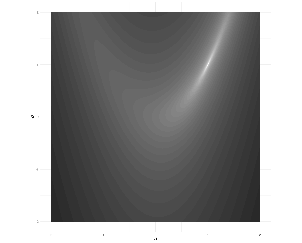
Here is the function definition. a and b are parameters that can be freely chosen; the values we use here are a frequent choice.
5.2 Minimization from scratch
The scenario is the following. We start at some given point (x1,x2), and set out to find the location where the Rosenbrock function has its minimum.
We follow the strategy outlined in the previous chapter: compute the function’s gradient at our current position, and use it to go the opposite way. We don’t know how far to go; if we take too big a big step we may easily overshoot. (If you look back at the contour plot, you see that if you were standing at one of the steep cliffs east or west of the minimum, this could happen very fast.)
Thus, it is best to proceed iteratively, taking moderate steps and re-evaluating the gradient every time.
In a nutshell, the optimization procedure then looks somewhat like this:
library(torch)

# attention: this is not the correct procedure yet!

for (i in 1:num_iterations) {

  # call function, passing in current parameter value
  value <- rosenbrock(x)

  # compute gradient of value w.r.t. parameter
  value$backward()

  # manually update parameter, subtracting a fraction
  # of the gradient
  # this is not quite correct yet!
  x$sub_(lr * x$grad)
}
As written, this code snippet demonstrates our intentions, but it’s not quite correct (yet). It is also missing a few prerequisites: Neither the tensor x nor the variables lr and num_iterations have been defined. Let’s make sure we have those ready first. lr, for learning rate, is the fraction of the gradient to subtract on every step, and num_iterations is the number of steps to take. Both are a matter of experimentation.
lr <- 0.01

num_iterations <- 1000
x is the parameter to optimize, that is, it is the function input that hopefully, at the end of the process, will yield the minimum possible function value. This makes it the tensor with respect to which we want to compute the function value’s derivative. And that, in turn, means we need to create it with requires_grad = TRUE:
x <- torch_tensor(c(-1, 1), requires_grad = TRUE)The starting point, (-1,1), here has been chosen arbitrarily.
Now, all that remains to be done is apply a small fix to the optimization loop. With autograd enabled on x, torch will record all operations performed on that tensor, meaning that whenever we call backward(), it will compute all required derivatives. However, when we subtract a fraction of the gradient, this is not something we want a derivative to be calculated for! We need to tell torch not to record this action, and that we can do by wrapping it in with_no_grad().
There’s one other thing we have to tell it. By default, torch accumulates the gradients stored in grad fields. We need to zero them out for every new calculation, using grad$zero_().
Taking into account these considerations, the parameter update should look like this:
with_no_grad({
  x$sub_(lr * x$grad)
  x$grad$zero_()
})
Here is the complete code, enhanced with logging statements that make it easier to see what is going on.
num_iterations <- 1000

lr <- 0.01

x <- torch_tensor(c(-1, 1), requires_grad = TRUE)

for (i in 1:num_iterations) {
  if (i %% 100 == 0) cat("Iteration: ", i, "\n")

  value <- rosenbrock(x)
  if (i %% 100 == 0) {
    cat("Value is: ", as.numeric(value), "\n")
  }

  value$backward()
  if (i %% 100 == 0) {
    cat("Gradient is: ", as.matrix(x$grad), "\n")
  }

  with_no_grad({
    x$sub_(lr * x$grad)
    x$grad$zero_()
  })
}
Iteration: 100
Value is: 0.3502924
Gradient is: -0.667685 -0.5771312
Iteration: 200
Value is: 0.07398106
Gradient is: -0.1603189 -0.2532476
Iteration: 300
Value is: 0.02483024
Gradient is: -0.07679074 -0.1373911
Iteration: 400
Value is: 0.009619333
Gradient is: -0.04347242 -0.08254051
Iteration: 500
Value is: 0.003990697
Gradient is: -0.02652063 -0.05206227
Iteration: 600
Value is: 0.001719962
Gradient is: -0.01683905 -0.03373682
Iteration: 700
Value is: 0.0007584976
Gradient is: -0.01095017 -0.02221584
Iteration: 800
Value is: 0.0003393509
Gradient is: -0.007221781 -0.01477957
Iteration: 900
Value is: 0.0001532408
Gradient is: -0.004811743 -0.009894371
Iteration: 1000
Value is: 6.962555e-05
Gradient is: -0.003222887 -0.006653666 After thousand iterations, we have reached a function value lower than 0.0001. What is the corresponding (x1,x2)-position?
xtorch_tensor
0.9918
0.9830
[ CPUFloatType{2} ]This is rather close to the true minimum of (1,1). If you feel like, play around a little, and try to find out what kind of difference the learning rate makes. For example, try 0.001 and 0.1, respectively.
In the next chapter, we will build a neural network from scratch. There, the function we minimize will be a loss function, namely, the mean squared error arising from a regression problem.