set.seed(777)

library(torch)
torch_manual_seed(777)

library(dplyr)
library(readr)

library(zeallot)

uci <- "https://archive.ics.uci.edu"
ds_path <- "ml/machine-learning-databases/00514"
ds_file <- "Bias_correction_ucl.csv"

# download.file(
#   file.path(uci, ds_path, ds_file),
#   destfile = "resources/matrix-weather.csv"
# )

weather_df <- read_csv("resources/matrix-weather.csv") %>%
  na.omit()
weather_df %>% glimpse()24 Matrix computations: Least-squares problems
In this chapter and the next, we’ll explore what torch lets us do with matrices. Here, we take a look at various ways to solve least-squares problems. The intention is two-fold.
Firstly, this subject often gets pretty technical, or rather, computational, very fast. Depending on your background (and goals), this may just be what you want; you either know well, or do not care about so much, the underlying concepts. But for some people, a purely technical presentation, one that does not also dwell on the concepts, the abstract ideas underlying the subject, may well fail to convey the fascination, the intellectual attraction it can exert. That’s why, in this chapter, I’ll try to present things in a way that the main ideas don’t get obscured by “computer-sciencey” details (details that are easily found in a number of excellent books, anyway).
24.1 Five ways to do least squares
How do you compute linear least-squares regression? In R, using lm(); in torch, there is linalg_lstsq(). Where R, sometimes, hides complexity from the user, high-performance computation frameworks like torch tend to ask a bit more up-front effort, be it careful reading of documentation, or playing around some, or both. For example, here is the central piece of documentation for linalg_lstsq(), elaborating on the driver parameter to the function:
driverchooses the LAPACK/MAGMA function that will be used.For CPU inputs the valid values are ‘gels’, ‘gelsy’, ‘gelsd, ’gelss’.
For CUDA input, the only valid driver is ‘gels’, which assumes that A is full-rank.
To choose the best driver on CPU consider:
- If A is well-conditioned (its condition number is not too large), or you do not mind some precision loss:
For a general matrix: ‘gelsy’ (QR with pivoting) (default)
If A is full-rank: ‘gels’ (QR)
- If A is not well-conditioned:
‘gelsd’ (tridiagonal reduction and SVD)
But if you run into memory issues: ‘gelss’ (full SVD).
Whether you’ll need to know this will depend on the problem you’re solving. But if you do, it certainly will help to have an idea what is being talked about there, if only in a high-level way.
In our example problem below, we’re going to be lucky. All drivers will return the same result – but only once we’ll have applied a “trick”, of sorts. Still, we’ll go on and dig deeper into the various methods used by linalg_lstsq(), as well as a few others of common use. Concretely, we’ll solve least squares:
By means of the so-called normal equations, the most direct way, in the sense that it immediately results from a mathematical statement of the problem.
Again, starting from the normal equations, but making use of Cholesky factorization in solving them.
Yet again, taking the normal equations for a point of departure, but proceeding by means of LU decomposition.
Fourth, employing another type of factorization – QR – that, together with the final one, accounts for the vast majority of decompositions applied “in the real world”. With QR decomposition, the solution algorithm does not start from the normal equations.
And fifth and finally, making use of Singular Value Decomposition (SVD). Here, too, the normal equations are not needed.
All methods will first be applied to a real-world dataset, and then, be tested on a benchmark problem well known for its lack of stability.
24.2 Regression for weather prediction
The dataset we’ll use is available from the UCI Machine Learning Repository. The way we’ll use it does not quite match the original purpose of collection; instead of forecasting temperature with machine learning, the original study (Cho et al. (2020)) really was about bias correction of forecasts obtained from a numerical weather prediction model. But never mind – our focus here is on matrix methods, and the dataset lends itself very well to the kinds of explorations we’re going to do.
Rows: 7,588
Columns: 25
$ station           <dbl> 1, 2, 3, 4, 5, 6, 7, 8, 9, 10, 11,…
$ Date              <date> 2013-06-30, 2013-06-30,…
$ Present_Tmax      <dbl> 28.7, 31.9, 31.6, 32.0, 31.4, 31.9,…
$ Present_Tmin      <dbl> 21.4, 21.6, 23.3, 23.4, 21.9, 23.5,…
$ LDAPS_RHmin       <dbl> 58.25569, 52.26340, 48.69048,…
$ LDAPS_RHmax       <dbl> 91.11636, 90.60472, 83.97359,…
$ LDAPS_Tmax_lapse  <dbl> 28.07410, 29.85069, 30.09129,…
$ LDAPS_Tmin_lapse  <dbl> 23.00694, 24.03501, 24.56563,…
$ LDAPS_WS          <dbl> 6.818887, 5.691890, 6.138224,…
$ LDAPS_LH          <dbl> 69.45181, 51.93745, 20.57305,…
$ LDAPS_CC1         <dbl> 0.2339475, 0.2255082, 0.2093437,…
$ LDAPS_CC2         <dbl> 0.2038957, 0.2517714, 0.2574694,…
$ LDAPS_CC3         <dbl> 0.1616969, 0.1594441, 0.2040915,…
$ LDAPS_CC4         <dbl> 0.1309282, 0.1277273, 0.1421253,…
$ LDAPS_PPT1        <dbl> 0.0000000, 0.0000000, 0.0000000,…
$ LDAPS_PPT2        <dbl> 0.000000, 0.000000, 0.000000,…
$ LDAPS_PPT3        <dbl> 0.0000000, 0.0000000, 0.0000000,…
$ LDAPS_PPT4        <dbl> 0.0000000, 0.0000000, 0.0000000,…
$ lat               <dbl> 37.6046, 37.6046, 37.5776, 37.6450,…
$ lon               <dbl> 126.991, 127.032, 127.058, 127.022,…
$ DEM               <dbl> 212.3350, 44.7624, 33.3068, 45.7160,…
$ Slope             <dbl> 2.7850, 0.5141, 0.2661, 2.5348,…
$ `Solar radiation` <dbl> 5992.896, 5869.312, 5863.556,…
$ Next_Tmax         <dbl> 29.1, 30.5, 31.1, 31.7, 31.2, 31.5,…
$ Next_Tmin         <dbl> 21.2, 22.5, 23.9, 24.3, 22.5, 24.0,…
The way we’re framing the task, basically everything in the dataset serves (or would serve, if we kept it – more on that below) as a predictor. As target, we’ll use Next_Tmax, the maximal temperature reached on the subsequent day. This means we need to remove Next_Tmin from the set of predictors, as it would make for too powerful of a clue. We’ll do the same for station, the weather station id, and Date. This leaves us with twenty-one predictors, including measurements of actual temperature (Present_Tmax, Present_Tmin), model forecasts of various variables (LDAPS_*), and auxiliary information (lat, lon, and `Solar radiation`, among others).
weather_df <- weather_df %>%
  select(-c(station, Next_Tmin, Date)) %>%
  mutate(across(.fns = scale))
Note how, above, I’ve added a line to standardize the predictors. This is the “trick” I was alluding to above. We’ll talk about why we’re doing this soon.
For torch, we split up the data into two tensors: a matrix A, containing all predictors, and a vector b that holds the target.
weather <- torch_tensor(weather_df %>% as.matrix())
A <- weather[ , 1:-2]
b <- weather[ , -1]

dim(A)
[1] 7588 21Now, first let’s determine the expected output.
24.2.1 Least squares (I): Setting expectations with lm()
If there’s a least squares implementation we “believe in”, it surely must be lm().
fit <- lm(Next_Tmax ~ . , data = weather_df)
fit %>% summary()
Call:
lm(formula = Next_Tmax ~ ., data = weather_df)
Residuals:
Min 1Q Median 3Q Max
-1.94439 -0.27097 0.01407 0.28931 2.04015
Coefficients:
Estimate Std. Error t value Pr(>|t|)
(Intercept) 2.605e-15 5.390e-03 0.000 1.000000
Present_Tmax 1.456e-01 9.049e-03 16.089 < 2e-16 ***
Present_Tmin 4.029e-03 9.587e-03 0.420 0.674312
LDAPS_RHmin 1.166e-01 1.364e-02 8.547 < 2e-16 ***
LDAPS_RHmax -8.872e-03 8.045e-03 -1.103 0.270154
LDAPS_Tmax_lapse 5.908e-01 1.480e-02 39.905 < 2e-16 ***
LDAPS_Tmin_lapse 8.376e-02 1.463e-02 5.726 1.07e-08 ***
LDAPS_WS -1.018e-01 6.046e-03 -16.836 < 2e-16 ***
LDAPS_LH 8.010e-02 6.651e-03 12.043 < 2e-16 ***
LDAPS_CC1 -9.478e-02 1.009e-02 -9.397 < 2e-16 ***
LDAPS_CC2 -5.988e-02 1.230e-02 -4.868 1.15e-06 ***
LDAPS_CC3 -6.079e-02 1.237e-02 -4.913 9.15e-07 ***
LDAPS_CC4 -9.948e-02 9.329e-03 -10.663 < 2e-16 ***
LDAPS_PPT1 -3.970e-03 6.412e-03 -0.619 0.535766
LDAPS_PPT2 7.534e-02 6.513e-03 11.568 < 2e-16 ***
LDAPS_PPT3 -1.131e-02 6.058e-03 -1.866 0.062056 .
LDAPS_PPT4 -1.361e-03 6.073e-03 -0.224 0.822706
lat -2.181e-02 5.875e-03 -3.713 0.000207 ***
lon -4.688e-02 5.825e-03 -8.048 9.74e-16 ***
DEM -9.480e-02 9.153e-03 -10.357 < 2e-16 ***
Slope 9.402e-02 9.100e-03 10.331 < 2e-16 ***
`Solar radiation` 1.145e-02 5.986e-03 1.913 0.055746 .
---
Signif. codes: 0 ‘***’ 0.001 ‘**’ 0.01 ‘*’ 0.05 ‘.’ 0.1 ‘ ’ 1
Residual standard error: 0.4695 on 7566 degrees of freedom
Multiple R-squared: 0.7802, Adjusted R-squared: 0.7796
F-statistic: 1279 on 21 and 7566 DF, p-value: < 2.2e-16With an explained variance of 78%, the forecast is working pretty well. This is the baseline we want to check all other methods against. To that purpose, we’ll store respective predictions and prediction errors (the latter being operationalized as root mean squared error, RMSE). For now, we just have entries for lm():
rmse <- function(y_true, y_pred) {
  (y_true - y_pred)^2 %>%
    sum() %>%
    sqrt()
}

all_preds <- data.frame(
  b = weather_df$Next_Tmax,
  lm = fit$fitted.values
)
all_errs <- data.frame(lm = rmse(all_preds$b, all_preds$lm))
all_errs
lm
1 40.836924.2.2 Least squares (II): Using linalg_lstsq()
Now, for a moment let’s assume this was not about exploring different approaches, but getting a quick result. In torch, we have linalg_lstsq(), a function dedicated specifically to solving least-squares problems. (This is the function whose documentation I was citing, above.) Just like we did with lm(), we’d probably just go ahead and call it, making use of the default settings:
x_lstsq <- linalg_lstsq(A, b)$solution

all_preds$lstsq <- as.matrix(A$matmul(x_lstsq))
all_errs$lstsq <- rmse(all_preds$b, all_preds$lstsq)

tail(all_preds)
b lm lstsq
7583 -1.1380931 -1.3544620 -1.3544616
7584 -0.8488721 -0.9040997 -0.9040993
7585 -0.7203294 -0.9675286 -0.9675281
7586 -0.6239224 -0.9044044 -0.9044040
7587 -0.5275154 -0.8738639 -0.8738635
7588 -0.7846007 -0.8725795 -0.8725792Predictions resemble those of lm() very closely – so closely, in fact, that we may guess those tiny differences are just due to numerical errors surfacing from deep down the respective call stacks. RMSE, thus, should be equal as well:
all_errs lm lstsq
1 40.8369 40.8369It is; and this is a satisfying outcome. However, it only really came about due to that “trick”: normalization. Of course, when I say “trick”, I don’t really mean it. Standardizing the data is a common operation, and especially with neural networks, it tends to get used routinely, to speed up training. The point I’d like to make is this: Frameworks for high-performance computation, like torch, will often presuppose more domain knowledge, or more up-front analysis, on the part of the user.
I’ll explain.
24.2.3 Interlude: What if we hadn’t standardized the data?
For quick comparison, let’s create an alternate matrix of predictors: not normalizing the data, this time.
weather_df_alt <-
  read_csv("resources/matrix-weather.csv") %>%
  na.omit() %>%
  select(-c(station, Next_Tmin, Date))

weather_alt <- torch_tensor(weather_df_alt %>% as.matrix())
A_alt <- weather_alt[ , 1:-2]
b_alt <- weather_alt[ , -1]
To set our expectations, we again call lm():
fit_alt <- lm(Next_Tmax ~ ., data = weather_df_alt)
all_preds_alt <- data.frame(
  b = weather_df_alt$Next_Tmax,
  lm = fit_alt$fitted.values
)

all_errs_alt <- data.frame(
  lm = rmse(
    all_preds_alt$b,
    all_preds_alt$lm
  )
)

all_errs_alt
lm
1 127.0765Now, we call linalg_lstsq(), using the default arguments just like we did before.
x_lstsq_alt <- linalg_lstsq(A_alt, b_alt)$solution

all_preds_alt$lstsq <- as.matrix(A_alt$matmul(x_lstsq_alt))
all_errs_alt$lstsq <- rmse(
  all_preds_alt$b, all_preds_alt$lstsq
)

all_errs_alt
lm lstsq
1 127.0765 177.9128Wow – what happened here? Thinking back of that piece of documentation I’ve cited, maybe the default arguments aren’t working out that well, this time. Let’s find out why.
24.2.3.1 Investigating “the issue”
To efficiently solve a linear least-squares problem, torch calls into LAPACK, a set of Fortran routines designed to efficiently and scaleably address the tasks most frequently found in linear algebra: solving linear systems of equations, computing eigenvectors and eigenvalues, and determining singular values.
The allowed drivers in linalg_lstsq() correspond to different LAPACK procedures1, and these procedures all apply different algorithms in order to solve the problem – analogously to what’ll we do ourselves, below.
Thus, in investigating what is going on, step one is to determine which method gets used and why; analyse (if possible) why the result is unsatisfying; determine the LAPACK routine we’d like to be using instead, and check what happens if indeed we do. (Of course, given the little effort involved, we’d probably give all methods a try.)
The main concept involved here is the rank of a matrix.
24.2.3.2 Concepts (I): Rank of a matrix
“But wait!” you may be thinking – from the above-cited piece of documentation, it seems like the first thing we should check is not rank, but condition number: whether the matrix is “well-conditioned”. Yes, the condition number certainly is important, and we’ll get back to it very soon. However, there is something even more fundamental at work here, something that does not really “jump to the eye”.
The central piece of information is found in that LAPACK piece of documentation we’re being referred to by linalg_lstsq(). Between the four routines GELS, GELSY, GELSD, and GELSS, differences are not restricted to implementation. The goal of optimization differs, as well. The rationale is the following. Throughout, let’s assume we’re working with a matrix that has more rows than columns (more observations than features, in the most-frequent case):
If the matrix is full-rank – meaning, its columns are linearly independent – there is no “perfect” solution. The problem is over-determined. All we can do is find the best possible approximation. This is done by minimizing the prediction error – we’ll come back to that when discussing the normal equations. Minimize prediction error is what the GELS routine does, and it is GELS we should use when we have a full-rank matrix of predictors.
If the matrix is not full-rank, the problem is under-determined; there is an infinite number of solutions. All the remaining routines – GELSY, GELSD, and GELSS – are suited to this situation. While they do proceed differently, they all pursue the same strategy, different from the one followed by GELS: In addition to the prediction error, they also minimize the vector of coefficients. This is called finding a minimum-norm least-squares solution.
In sum, GELS (for full-rank matrices) and the three of GELSY, GELSD, and GELSS (for when the matrix is rank-deficient) intentionally follow different optimization criteria.
Now, as per the documentation for linalg_lstsq(), when no driver is passed explicitly, it is GELSY that gets called. That should be fine if our matrix is rank-deficient – but is it?
linalg_matrix_rank(A_alt)torch_tensor
21
[ CPULongType{} ]The matrix has twenty-one columns; so if its rank is twenty-one, then it is full-rank for sure. We definitely want to be calling the GELS routine.
24.2.3.3 Calling linalg_lstsq() the right way
Now that we know what to pass for driver, here is the modified call:
x_lstsq_alt <- linalg_lstsq(
  A_alt, b_alt,
  driver = "gels"
)$solution

all_preds_alt$lstsq <- as.matrix(A_alt$matmul(x_lstsq_alt))
all_errs_alt$lstsq <- rmse(
  all_preds_alt$b,
  all_preds_alt$lstsq
)

all_errs_alt
lm lstsq
1 127.0765 127.9489Now, the respective RMSE values are very close. You’ll be wondering, though: Why didn’t we have to specify the Fortran routine when working with the standardized matrix?
24.2.3.4 Why did standardization help?
For our matrix, what standardization did was reduce significantly the range spanned by the singular values. With A, the standardized matrix, the largest singular value is about ten times as large as the smallest one:
svals_normalized_A <- linalg_svdvals(A)/linalg_svdvals(A)[1]
svals_normalized_A %>% as.numeric()
[1] 1.0000000 0.7473214 0.5929527 0.5233989 0.5188764 0.4706140
[7] 0.4391665 0.4249273 0.4034659 0.3815900 0.3621315 0.3557949
[13] 0.3297923 0.2707912 0.2489560 0.2229859 0.2175170 0.1852890
[19] 0.1627083 0.1553169 0.1075778While with A_alt, it is a million times as large:
svals_normalized_A_alt <- linalg_svdvals(A_alt) /
  linalg_svdvals(A_alt)[1]
svals_normalized_A_alt %>% as.numeric()
[1] 1.000000e+00 1.014369e-02 6.407313e-03 2.881966e-03
[5] 2.236537e-03 9.633782e-04 6.678377e-04 3.988165e-04
[9] 3.584047e-04 3.137257e-04 2.699152e-04 2.383501e-04
[13] 2.234150e-04 1.803384e-04 1.625245e-04 1.300101e-04
[17] 4.312536e-05 3.463851e-05 1.964120e-05 1.689913e-05
[18] 8.419599e-06Why is this important? It’s here that we finally get back to the condition number.
24.2.3.5 Concepts (II): Condition number
The higher the so-called condition number of a matrix, the more likely we are to run into problems of numerical stability when computing with it. In torch, linalg_cond() is used to obtain the condition number. Let’s compare the condition numbers for A and A_alt, respectively.
linalg_cond(A)
linalg_cond(A_alt)
torch_tensor
9.2956
[ CPUFloatType{} ]
torch_tensor
118770
[ CPUFloatType{} ]That is quite a difference! How does it arise?
The condition number is defined as the matrix norm of A, divided by the norm of its inverse. Different kinds of norm may be used; the default is the 2-norm. In this case, condition number can be computed from the matrix’s singular values: Namely, the 2-norm of A equals the largest singular value, while that of its inverse is given by the smallest one.
We can verify this ourselves, using linalg_svdvals() as before:
linalg_svdvals(A)[1]/linalg_svdvals(A)[21]
linalg_svdvals(A_alt)[1]/linalg_svdvals(A_alt)[21]
torch_tensor
9.29559
[ CPUFloatType{} ]
torch_tensor
118770
[ CPUFloatType{} ]To reiterate, this is a substantial difference. Incidentally, do you remember that in the case of A_alt, RMSE was a tiny bit worse for linalg_lstsq() than for lm(), even when using the appropriate routine, GELS? Given that both essentially use the same algorithm (QR factorization, to be introduced very soon) this may very well have been due to numerical errors, arising from the high condition number of A_alt.
By now, I may have convinced you that with torch’s linalg component, it helps to know a bit about how the most-in-use least-squares algorithms work. Let’s get acquainted.
24.2.4 Least squares (III): The normal equations
We start by stating the goal. Given a matrix, \(\mathbf{A}\), that holds features in its columns and observations in its rows, and a vector of observed outcomes, \(\mathbf{b}\), we want to find regression coefficients, one for each feature, that allow to approximate \(\mathbf{b}\) as well as possible. Call the vector of regression coefficients \(\mathbf{x}\). To obtain it, we need to solve a simultaneous system of equations, that in matrix notation appears as
\[ \mathbf{Ax} = \mathbf{b} \]
If \(\mathbf{b}\) were a square, invertible matrix, the solution could directly be computed as \(\mathbf{x} = \mathbf{A}^{-1}\mathbf{b}\). This will hardly ever be possible, though; we’ll (hopefully) always have more observations than predictors. Another approach is needed. It directly starts from the problem statement.
When we use the columns of \(\mathbf{A}\) to approximate \(\mathbf{b}\), that approximation necessarily is in the column space of \(\mathbf{A}\). \(\mathbf{b}\), on the other hand, normally won’t be. We want those two to be as close as possible; in other words, we want to minimize the distance between them. Choosing the 2-norm for the distance, this yields the objective
\[ minimize \ ||\mathbf{Ax}-\mathbf{b}||^2 \]
This distance is the (squared) length of the vector of prediction errors. That vector necessarily is orthogonal to \(\mathbf{A}\) itself. That is, when we multiply it with \(\mathbf{A}\), we get the zero vector:
\[ \mathbf{A}^T(\mathbf{Ax} - \mathbf{b}) = \mathbf{0} \]
A rearrangement of this equation yields the so-called normal equations:
\[ \mathbf{A}^T \mathbf{A} \mathbf{x} = \mathbf{A}^T \mathbf{b} \]
These may be solved for \(\mathbf{x}\), computing the inverse of \(\mathbf{A}^T\mathbf{A}\):
\[ \mathbf{x} = (\mathbf{A}^T \mathbf{A})^{-1} \mathbf{A}^T \mathbf{b} \]
\(\mathbf{A}^T\mathbf{A}\) is a square matrix. It still might not be invertible, in which case the so-called pseudoinverse would be computed instead. In our case, this will not be needed; we already know \(\mathbf{A}\) has full rank, and so does \(\mathbf{A}^T\mathbf{A}\).
Thus, from the normal equations we have derived a recipe for computing \(\mathbf{b}\). Let’s put it to use, and compare with what we got from lm() and linalg_lstsq().
AtA <- A$t()$matmul(A)
Atb <- A$t()$matmul(b)
inv <- linalg_inv(AtA)
x <- inv$matmul(Atb)

all_preds$neq <- as.matrix(A$matmul(x))
all_errs$neq <- rmse(all_preds$b, all_preds$neq)

all_errs
lm lstsq neq
1 40.8369 40.8369 40.8369Having confirmed that the direct way works, we may allow ourselves some sophistication. Four different matrix factorizations will make their appearance: Cholesky, LU, QR, and Singular Value Decomposition. The goal, in every case, is to avoid the expensive computation of the (pseudo-) inverse. That’s what all methods have in common. However, they do not differ “just” in the way the matrix is factorized, but also, in which matrix is. This has to do with the constraints the various methods impose. Roughly speaking, the order they’re listed in above reflects a falling slope of preconditions, or put differently, a rising slope of generality. Due to the constraints involved, the first two (Cholesky, as well as LU decomposition) will be performed on \(\mathbf{A}^T\mathbf{A}\), while the latter two (QR and SVD) operate on \(\mathbf{A}\) directly. With them, there never is a need to compute \(\mathbf{A}^T\mathbf{A}\).
24.2.5 Least squares (IV): Cholesky decomposition
In Cholesky decomposition, a matrix is factored into two triangular matrices of the same size, with one being the transpose of the other. This commonly is written either
\[ \mathbf{A} = \mathbf{L} \mathbf{L}^T \] or
\[ \mathbf{A} = \mathbf{R}^T\mathbf{R} \]
Here symbols \(\mathbf{L}\) and \(\mathbf{R}\) denote lower-triangular and upper-triangular matrices, respectively.
For Cholesky decomposition to be possible, a matrix has to be both symmetric and positive definite. These are pretty strong conditions, ones that will not often be fulfilled in practice. In our case, \(\mathbf{A}\) is not symmetric; this immediately implies we have to operate on \(\mathbf{A}^T\mathbf{A}\) instead. And since \(\mathbf{A}\) already is positive definite, we know that \(\mathbf{A}^T\mathbf{A}\) is, as well.
In torch, we obtain the Cholesky decomposition of a matrix using linalg_cholesky(). By default, this call will return \(\mathbf{L}\), a lower-triangular matrix.
# AtA = L L_t
AtA <- A$t()$matmul(A)
L <- linalg_cholesky(AtA)
Let’s check that we can reconstruct \(\mathbf{A}\) from \(\mathbf{L}\):
LLt <- L$matmul(L$t())
diff <- LLt - AtA
linalg_norm(diff, ord = "fro")
torch_tensor
0.00258896
[ CPUFloatType{} ]Here, I’ve computed the Frobenius norm of the difference between the original matrix and its reconstruction. The Frobenius norm individually sums up all matrix entries, and returns the square root. In theory, we’d like to see zero here; but in the presence of numerical errors, the result is sufficient to indicate that the factorization worked fine.
Now that we have \(\mathbf{L}\mathbf{L}^T\) instead of \(\mathbf{A}^T\mathbf{A}\), how does that help us? It’s here that the magic happens, and you’ll find the same type of magic at work in the remaining three methods. The idea is that due to some decomposition, a more performant way arises of solving the system of equations that constitute a given task.
With \(\mathbf{L}\mathbf{L}^T\), the point is that \(\mathbf{L}\) is triangular, and when that’s the case the linear system can be solved by simple substitution. That is best visible with a tiny example:
\[ \begin{bmatrix} 1 & 0 & 0\\ 2 & 3 & 0\\ 3 & 4 & 1 \end{bmatrix} \begin{bmatrix} x1\\ x2\\ x3 \end{bmatrix} = \begin{bmatrix} 1\\ 11\\ 15 \end{bmatrix} \]
Starting in the top row, we immediately see that \(x1\) equals \(1\); and once we know that it is straightforward to calculate, from row two, that \(x2\) must be \(3\). The last row then tells us that \(x3\) must be \(0\).
In code, torch_triangular_solve() is used to efficiently compute the solution to a linear system of equations where the matrix of predictors is lower- or upper-triangular. An additional requirement is for the matrix to be symmetric – but that condition we already had to satisfy in order to be able to use Cholesky factorization.
By default, torch_triangular_solve() expects the matrix to be upper- (not lower-)triangular; but there is a function parameter, upper, that lets us correct that expectation. The return value is a list, and its first item contains the desired solution. To illustrate, here is torch_triangular_solve(), applied to the toy example we manually solved above:
some_L <- torch_tensor(
  matrix(c(1, 0, 0, 2, 3, 0, 3, 4, 1), nrow = 3, byrow = TRUE)
)
some_b <- torch_tensor(matrix(c(1, 11, 15), ncol = 1))

x <- torch_triangular_solve(
  some_b,
  some_L,
  upper = FALSE
)[[1]]
x
torch_tensor
1
3
0
[ CPUFloatType{3,1} ]Returning to our running example, the normal equations now look like this:
\[ \mathbf{L}\mathbf{L}^T \mathbf{x} = \mathbf{A}^T \mathbf{b} \]
We introduce a new variable, \(\mathbf{y}\), to stand for \(\mathbf{L}^T \mathbf{x}\),
\[ \mathbf{L}\mathbf{y} = \mathbf{A}^T \mathbf{b} \]
and compute the solution to this system:
Atb <- A$t()$matmul(b)

y <- torch_triangular_solve(
  Atb$unsqueeze(2),
  L,
  upper = FALSE
)[[1]]
Now that we have \(y\), we look back at how it was defined:
\[ \mathbf{y} = \mathbf{L}^T \mathbf{x} \]
To determine \(\mathbf{x}\), we can thus again use torch_triangular_solve():
x <- torch_triangular_solve(y, L$t())[[1]]And there we are.
As usual, we compute the prediction error:
all_preds$chol <- as.matrix(A$matmul(x))
all_errs$chol <- rmse(all_preds$b, all_preds$chol)

all_errs
lm lstsq neq chol
1 40.8369 40.8369 40.8369 40.8369Now that you’ve seen the rationale behind Cholesky factorization – and, as already suggested, the idea carries over to all other decompositions – you might like to save yourself some work making use of a dedicated convenience function, torch_cholesky_solve(). This will render obsolete the two calls to torch_triangular_solve().
The following lines yield the same output as the code above – but, of course, they do hide the underlying magic.
L <- linalg_cholesky(AtA)

x <- torch_cholesky_solve(Atb$unsqueeze(2), L)

all_preds$chol2 <- as.matrix(A$matmul(x))
all_errs$chol2 <- rmse(all_preds$b, all_preds$chol2)
all_errs
lm lstsq neq chol chol2
1 40.8369 40.8369 40.8369 40.8369 40.8369Let’s move on to the next method – equivalently, to the next factorization.
24.2.6 Least squares (V): LU factorization
LU factorization is named after the two factors it introduces: a lower-triangular matrix, \(\mathbf{L}\), as well as an upper-triangular one, \(\mathbf{U}\). In theory, there are no restrictions on LU decomposition: Provided we allow for row exchanges, effectively turning \(\mathbf{A} = \mathbf{L}\mathbf{U}\) into \(\mathbf{A} = \mathbf{P}\mathbf{L}\mathbf{U}\) (where \(\mathbf{P}\) is a permutation matrix), we can factorize any matrix.
In practice, though, if we want to make use of torch_triangular_solve() , the input matrix has to be symmetric. Therefore, here too we have to work with \(\mathbf{A}^T\mathbf{A}\), not \(\mathbf{A}\) directly. (And that’s why I’m showing LU decomposition right after Cholesky – they’re similar in what they make us do, though not at all similar in spirit.)
Working with \(\mathbf{A}^T\mathbf{A}\) means we’re again starting from the normal equations. We factorize \(\mathbf{A}^T\mathbf{A}\), then solve two triangular systems to arrive at the final solution. Here are the steps, including the not-always-needed permutation matrix \(\mathbf{P}\):
\[ \begin{aligned} \mathbf{A}^T \mathbf{A} \mathbf{x} &= \mathbf{A}^T \mathbf{b} \\ \mathbf{P} \mathbf{L}\mathbf{U} \mathbf{x} &= \mathbf{A}^T \mathbf{b} \\ \mathbf{L} \mathbf{y} &= \mathbf{P}^T \mathbf{A}^T \mathbf{b} \\ \mathbf{y} &= \mathbf{U} \mathbf{x} \end{aligned} \]
We see that when \(\mathbf{P}\) is needed, there is an additional computation: Following the same strategy as we did with Cholesky, we want to move \(\mathbf{P}\) from the left to the right. Luckily, what may look expensive – computing the inverse – is not: For a permutation matrix, its transpose reverses the operation.
Code-wise, we’re already familiar with most of what we need to do. The only missing piece is torch_lu(). torch_lu() returns a list of two tensors, the first a compressed representation of the three matrices \(\mathbf{P}\), \(\mathbf{L}\), and \(\mathbf{U}\). We can uncompress it using torch_lu_unpack() :
lu <- torch_lu(AtA)

c(P, L, U) %<-% torch_lu_unpack(lu[[1]], lu[[2]])
We move \(\mathbf{P}\) to the other side:
Atb <- P$t()$matmul(Atb)All that remains to be done is solve two triangular systems, and we are done:
y <- torch_triangular_solve(
  Atb$unsqueeze(2),
  L,
  upper = FALSE
)[[1]]
x <- torch_triangular_solve(y, U)[[1]]

all_preds$lu <- as.matrix(A$matmul(x))
all_errs$lu <- rmse(all_preds$b, all_preds$lu)
all_errs[1, -5]
lm lstsq neq chol lu
1 40.8369 40.8369 40.8369 40.8369 40.8369As with Cholesky decomposition, we can save ourselves the trouble of calling torch_triangular_solve() twice. torch_lu_solve() takes the decomposition, and directly returns the final solution:
lu <- torch_lu(AtA)
x <- torch_lu_solve(Atb$unsqueeze(2), lu[[1]], lu[[2]])

all_preds$lu2 <- as.matrix(A$matmul(x))
all_errs$lu2 <- rmse(all_preds$b, all_preds$lu2)
all_errs[1, -5]
lm lstsq neq chol lu lu
1 40.8369 40.8369 40.8369 40.8369 40.8369 40.8369Now, we look at the two methods that don’t require computation of \(\mathbf{A}^T\mathbf{A}\).
24.2.7 Least squares (VI): QR factorization
Any matrix can be decomposed into an orthogonal matrix, \(\mathbf{Q}\), and an upper-triangular matrix, \(\mathbf{R}\). QR factorization is probably the most popular approach to solving least-squares problems; it is, in fact, the method used by R’s lm(). In what ways, then, does it simplify the task?
As to \(\mathbf{R}\), we already know how it is useful: By virtue of being triangular, it defines a system of equations that can be solved step-by-step, by means of mere substitution. \(\mathbf{Q}\) is even better. An orthogonal matrix is one whose columns are orthogonal – meaning, mutual dot products are all zero – and have unit norm; and the nice thing about such a matrix is that its inverse equals its transpose. In general, the inverse is hard to compute; the transpose, however, is easy. Seeing how computation of an inverse – solving \(\mathbf{x}=\mathbf{A}^{-1}\mathbf{b}\) – is just the central task in least squares, it’s immediately clear how significant this is.
Compared to our usual scheme, this leads to a slightly shortened recipe. There is no “dummy” variable \(\mathbf{y}\) anymore. Instead, we directly move \(\mathbf{Q}\) to the other side, computing the transpose (which is the inverse). All that remains, then, is back-substitution. Also, since every matrix has a QR decomposition, we now directly start from \(\mathbf{A}\) instead of \(\mathbf{A}^T\mathbf{A}\):
\[ \begin{aligned} \mathbf{A}\mathbf{x} &= \mathbf{b}\\ \mathbf{Q}\mathbf{R}\mathbf{x} &= \mathbf{b}\\ \mathbf{R}\mathbf{x} &= \mathbf{Q}^T\mathbf{b}\\ \end{aligned} \]
In torch, linalg_qr() gives us the matrices \(\mathbf{Q}\) and \(\mathbf{R}\).
c(Q, R) %<-% linalg_qr(A)On the right side, we used to have a “convenience variable” holding \(\mathbf{A}^T\mathbf{b}\) ; here, we skip that step, and instead, do something “immediately useful”: move \(\mathbf{Q}\) to the other side.
Qtb <- Q$t()$matmul(b)The only remaining step now is to solve the remaining triangular system.
x <- torch_triangular_solve(Qtb$unsqueeze(2), R)[[1]]

all_preds$qr <- as.matrix(A$matmul(x))
all_errs$qr <- rmse(all_preds$b, all_preds$qr)
all_errs[1, -c(5,7)]
lm lstsq neq chol lu qr
1 40.8369 40.8369 40.8369 40.8369 40.8369 40.8369 By now, you’ll be expecting for me to end this section saying “there is also a dedicated solver in torch/torch_linalg, namely …”). Well, not literally, no; but effectively, yes. If you call linalg_lstsq() passing driver = "gels", it is QR factorization that will be used.
24.2.8 Least squares (VII): Singular Value Decomposition (SVD)
In true climactic order, the last factorization method we discuss is the most versatile, most diversely applicable, most semantically meaningful one: Singular Value Decomposition (SVD). The third aspect, fascinating though it is, does not relate to our current task, so I won’t go into it here. Here, it is universal applicability that matters: Every matrix can be composed into components SVD-style.
Singular Value Decomposition factors an input \(\mathbf{A}\) into two orthogonal matrices, called \(\mathbf{U}\) and \(\mathbf{V}^T\), and a diagonal one, named \(\symbf{\Sigma}\), such that \(\mathbf{A} = \mathbf{U} \symbf{\Sigma} \mathbf{V}^T\). Here \(\mathbf{U}\) and \(\mathbf{V}^T\) are the left and right singular vectors, and \(\symbf{\Sigma}\) holds the singular values.
\[ \begin{aligned} \mathbf{A}\mathbf{x} &= \mathbf{b}\\ \mathbf{U}\symbf{\Sigma}\mathbf{V}^T\mathbf{x} &= \mathbf{b}\\ \symbf{\Sigma}\mathbf{V}^T\mathbf{x} &= \mathbf{U}^T\mathbf{b}\\ \mathbf{V}^T\mathbf{x} &= \mathbf{y}\\ \end{aligned} \]
We start by obtaining the factorization, using linalg_svd() . The argument full_matrices = FALSE tells torch that we want a \(\mathbf{U}\) of dimensionality same as \(\mathbf{A}\), not expanded to 7588 x 7588.
c(U, S, Vt) %<-% linalg_svd(A, full_matrices = FALSE)

dim(U)
dim(S)
dim(Vt)
[1] 7588 21
[1] 21
[1] 21 21We move \(\mathbf{U}\) to the other side – a cheap operation, thanks to \(\mathbf{U}\) being orthogonal.
Utb <- U$t()$matmul(b)With both \(\mathbf{U}^T\mathbf{b}\) and \(\symbf{\Sigma}\) being same-length vectors, we can use element-wise multiplication to do the same for \(\symbf{\Sigma}\). We introduce a temporary variable, y, to hold the result.
y <- Utb / SNow left with the final system to solve, \(\mathbf{\mathbf{V}^T\mathbf{x} = \mathbf{y}}\), we again profit from orthogonality – this time, of the matrix \(\mathbf{V}^T\).
x <- Vt$t()$matmul(y)Wrapping up, let’s calculate predictions and prediction error:
all_preds$svd <- as.matrix(A$matmul(x))
all_errs$svd <- rmse(all_preds$b, all_preds$svd)

all_errs[1, -c(5, 7)]
lm lstsq neq chol lu qr svd
1 40.8369 40.8369 40.8369 40.8369 40.8369 40.8369 40.8369That concludes our tour of important least-squares algorithms. Wrapping up the example, we take a quick look at performance.
24.2.9 Checking execution times
Like I said, the focus in this chapter is on concepts, not performance. But once you work with bigger datasets, you inevitably will care about speed. Also, it’s just interesting to see how fast those methods are! So, let’s do a quick performance benchmark. Just, please, don’t extrapolate from these results – instead, run analogous code on the data you care about.
To time them, we need all algorithms encapsulated in their respective functions. Here they are:
# normal equations
ls_normal_eq <- function(A, b) {
  AtA <- A$t()$matmul(A)
  x <- linalg_inv(AtA)$matmul(A$t())$matmul(b)
  x
}

# normal equations and Cholesky decomposition (done manually)
# A_t A x = A_t b
# L L_t x = A_t b
# L y = A_t b
# L_t x = y
ls_cholesky_diy <- function(A, b) {
  AtA <- A$t()$matmul(A)
  Atb <- A$t()$matmul(b)
  L <- linalg_cholesky(AtA)
  y <- torch_triangular_solve(
    Atb$unsqueeze(2),
    L,
    upper = FALSE
  )[[1]]
  x <- torch_triangular_solve(y, L$t())[[1]]
  x
}

# torch's Cholesky solver
ls_cholesky_solve <- function(A, b) {
  AtA <- A$t()$matmul(A)
  Atb <- A$t()$matmul(b)
  L <- linalg_cholesky(AtA)
  x <- torch_cholesky_solve(Atb$unsqueeze(2), L)
  x
}

# normal equations and LU factorization (done manually)
# A_t A x = A_t b
# P L U x = A_t b
# L y = P_t A_t b          # where y = U x
# U x = y
ls_lu_diy <- function(A, b) {
  AtA <- A$t()$matmul(A)
  Atb <- A$t()$matmul(b)
  lu <- torch_lu(AtA)
  c(P, L, U) %<-% torch_lu_unpack(lu[[1]], lu[[2]])
  Atb <- P$t()$matmul(Atb)
  y <- torch_triangular_solve(
    Atb$unsqueeze(2),
    L,
    upper = FALSE
  )[[1]]
  x <- torch_triangular_solve(y, U)[[1]]
  x
}

# torch's LU solver
ls_lu_solve <- function(A, b) {
  AtA <- A$t()$matmul(A)
  Atb <- A$t()$matmul(b)
  lu <- torch_lu(AtA)
  m = lu[[1]]
  pivots = lu[[2]]
  x <- torch_lu_solve(Atb$unsqueeze(2), m, pivots)
  x
}

# QR factorization
# A x = b
# Q R x = b
# R x = Q_t b
ls_qr <- function(A, b) {
  c(Q, R) %<-% linalg_qr(A)
  Qtb <- Q$t()$matmul(b)
  x <- torch_triangular_solve(Qtb$unsqueeze(2), R)[[1]]
  x
}

# SVD
# A x = b
# U S V_ x = b
# S V_t x = U_t b
# S y = U_t b
# V_t x = y
ls_svd <- function(A, b) {
  c(U, S, Vt) %<-% linalg_svd(A, full_matrices = FALSE)
  Utb <- U$t()$matmul(b)
  y <- Utb / S
  x <- Vt$t()$matmul(y)
  x
}

# torch's general least squares solver
ls_lstsq <- function(A, b) {
  x <- linalg_lstsq(A, b)
  x
}
We use the bench package to profile those methods. The mark() function does a lot more than just track time; however, here we just take a glance at the distributions of execution times (fig. 24.1):
set.seed(777)
torch_manual_seed(777)
library(bench)
library(ggplot2)

res <- mark(ls_normal_eq(A, b),
            ls_cholesky_diy(A, b),
            ls_cholesky_solve(A, b),
            ls_lu_diy(A, b),
            ls_lu_solve(A, b),
            ls_qr(A, b),
            ls_svd(A, b),
            ls_lstsq(A, b)$solution,
            min_iterations = 1000)

autoplot(res, type = "ridge") + theme_minimal()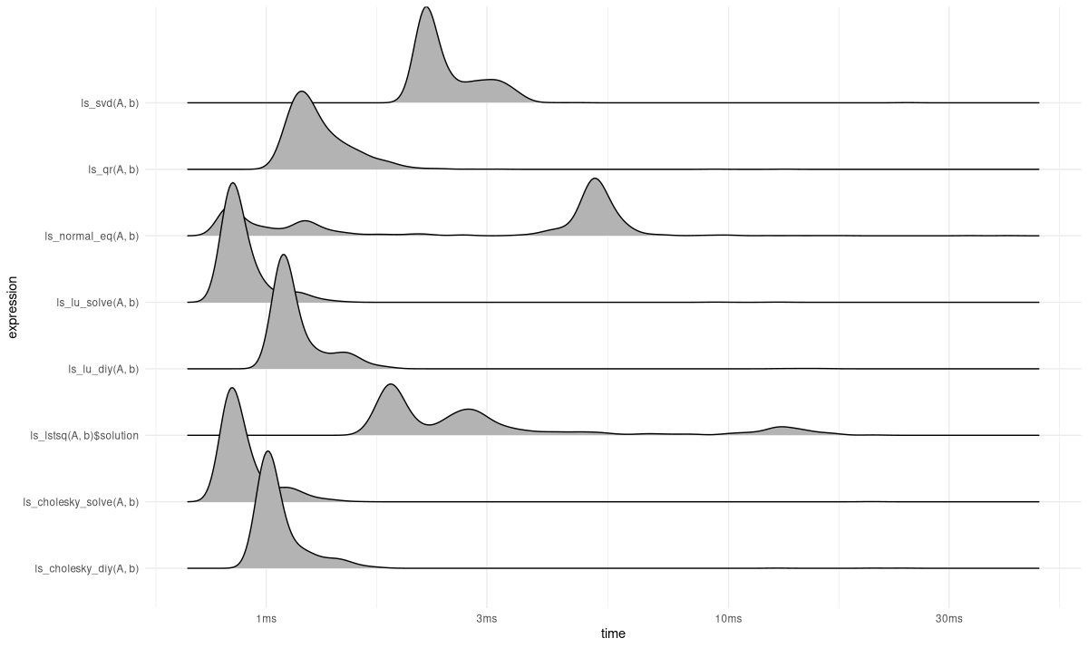
In conclusion, we saw how different ways of factorizing a matrix can help in solving least squares problems. We also quickly showed a way to time those strategies; however, speed is not all that counts. We want the solution to be reliable, as well. The technical term here is stability.
24.3 A quick look at stability
We’ve already talked about condition numbers. The concept of stability is similar in spirit, but refers to an algorithm instead of a matrix. In both cases, the idea is that small changes in the input to a calculation should lead to small changes in the output. Whole books have been dedicated to this topic, so I’ll refrain from going into details2.
Instead, I’ll use an example of an ill-conditioned least-squares problem – meaning, the matrix is ill-conditioned – for us to form an idea about the stability of the algorithms we’ve discussed3.
The matrix of predictors is a 100 x 15 Vandermonde matrix, created like so:
set.seed(777)
torch_manual_seed(777)

m <- 100
n <- 15
t <- torch_linspace(0, 1, m)$to(dtype = torch_double())

A <- torch_vander(t, N = n, increasing = TRUE)$to(
  dtype = torch_double()
)
Condition number is very high:
linalg_cond(A)torch_tensor
2.27178e+10
[ CPUDoubleType{} ]Even higher is the condition number obtained when we multiply it with its transpose – remember that some algorithms actually need to work with this matrix:
linalg_cond(A$t()$matmul(A))torch_tensor
7.27706e+17
[ CPUDoubleType{} ]Next, we have the prediction target:
b <- torch_exp(torch_sin(4*t))
b <- b/2006.787453080206
In our example above, we ended up with the same RMSE for all methods. It will be interesting to see what happens here. I’ll restrict myself to the “DIY” ones among the methods shown before. Here they are, listed again for convenience:
# normal equations
ls_normal_eq <- function(A, b) {
  AtA <- A$t()$matmul(A)
  x <- linalg_inv(AtA)$matmul(A$t())$matmul(b)
  x
}

# normal equations and Cholesky decomposition (done manually)
# A_t A x = A_t b
# L L_t x = A_t b
# L y = A_t b
# L_t x = y
ls_cholesky_diy <- function(A, b) {
  # add a small multiple of the identity matrix
  # to counteract numerical instability
  # if Cholesky decomposition fails in your
  # setup, increase eps
  eps <- 1e-10
  id <- eps * torch_diag(torch_ones(dim(A)[2]))
  AtA <- A$t()$matmul(A) + id
  Atb <- A$t()$matmul(b)
  L <- linalg_cholesky(AtA)
  y <- torch_triangular_solve(
    Atb$unsqueeze(2),
    L,
    upper = FALSE
  )[[1]]
  x <- torch_triangular_solve(y, L$t())[[1]]
  x
}

# normal equations and LU factorization (done manually)
# A_t A x = A_t b
# P L U x = A_t b
# L y = P_t A_t b          # where y = U x
# U x = y
ls_lu_diy <- function(A, b) {
  AtA <- A$t()$matmul(A)
  Atb <- A$t()$matmul(b)
  lu <- torch_lu(AtA)
  c(P, L, U) %<-% torch_lu_unpack(lu[[1]], lu[[2]])
  Atb <- P$t()$matmul(Atb)
  y <- torch_triangular_solve(
    Atb$unsqueeze(2),
    L,
    upper = FALSE
  )[[1]]
  x <- torch_triangular_solve(y, U)[[1]]
  x
}

# QR factorization
# A x = b
# Q R x = b
# R x = Q_t b
ls_qr <- function(A, b) {
  c(Q, R) %<-% linalg_qr(A)
  Qtb <- Q$t()$matmul(b)
  x <- torch_triangular_solve(Qtb$unsqueeze(2), R)[[1]]
  x
}

# SVD
# A x = b
# U S V_ x = b
# S V_t x = U_t b
# S y = U_t b
# V_t x = y
ls_svd <- function(A, b) {
  c(U, S, Vt) %<-% linalg_svd(A, full_matrices = FALSE)
  Utb <- U$t()$matmul(b)
  y <- Utb / S
  x <- Vt$t()$matmul(y)
  x
}
Let’s see, then!
algorithms <- c(
  "ls_normal_eq",
  "ls_cholesky_diy",
  "ls_lu_diy",
  "ls_qr",
  "ls_svd"
)

rmses <- purrr::map(
  algorithms,
  function(m) {
    rmse(
      as.numeric(b),
      as.numeric(A$matmul(get(m)(A, b)))
    )
  }
)

rmse_df <- data.frame(
  method = algorithms,
  rmse = unlist(rmses)
)

rmse_df
method rmse
1 ls_normal_eq 2.882399e-03
2 ls_cholesky_diy 1.373906e-06
3 ls_lu_diy 1.274305e-07
4 ls_qr 3.436749e-08
5 ls_svd 3.436749e-08This is pretty impressive! We clearly see how the normal equations, straightforward though they are, may not be the best option once problems cease to be well-conditioned. Cholesky as well as LU decomposition fare better; however, the clear “winners” are QR factorization and the SVD. No wonder those two (with two variants each) are the ones made use of by linalg_lstsq().
The documentation for
drivercited above is basically an excerpt from the corresponding documentation in LAPACK, as we can easily verify, since the page in question has conveniently been linked in the documentation forlinalg_lstsq().↩︎To learn more, consider consulting one of those books, for example, the widely-used (and concise) treatment by Trefethen and Bau (1997).↩︎
The example is taken from the book by Trefethen and Bau referred to in the footnote above. Credits to Rachel Thomas, who brought this to my attention by virtue of using it in her numerical linear algebra course.↩︎