library(torch)
library(torchvision)
library(luz)

convnet <- nn_module(
  "convnet",
  initialize = function() {
    # nn_conv2d(in_channels, out_channels, kernel_size, stride)
    self$conv1 <- nn_conv2d(1, 32, 3, 1)
    self$conv2 <- nn_conv2d(32, 64, 3, 2)
    self$conv3 <- nn_conv2d(64, 128, 3, 1)
    self$conv4 <- nn_conv2d(128, 256, 3, 2)
    self$conv5 <- nn_conv2d(256, 10, 3, 2)

    self$bn1 <- nn_batch_norm2d(32)
    self$bn2 <- nn_batch_norm2d(64)
    self$bn3 <- nn_batch_norm2d(128)
    self$bn4 <- nn_batch_norm2d(256)
  },
  forward = function(x) {
    x %>%
      self$conv1() %>%
      nn_relu() %>%
      self$bn1() %>%
      self$conv2() %>%
      nn_relu() %>%
      self$bn2() %>%
      self$conv3() %>%
      nn_relu() %>%
      self$bn3() %>%
      self$conv4() %>%
      nn_relu() %>%
      self$bn4() %>%
      self$conv5() %>%
      torch_squeeze()
  }
)17 Speeding up training
You could say that the topics discussed in this and the preceding chapter relate like the non-negotiable and the desirable. Generalization, the ability to abstract over individual instances, is a sine qua non of a good model; however, we need to arrive at such a model in reasonable time (where reasonable means very different things in different contexts).
This time, in presenting techniques I’ll follow a different strategy, ordering them not by stages in the workflow, but by increasing generality. We’ll be looking at three very different, very successful (each in its own way) ideas:
Batch normalization. Batchnorm – to introduce a popular abbreviation – layers are added to a model to stabilize and, in consequence, speed up training.
Determining a good learning rate upfront, and dynamically varying it during training. As you might remember from our experiments with optimization, the learning rate has an enormous impact on training speed and stability.
Transfer learning. Applied to neural networks, the term commonly refers to using pre-trained models for feature detection, and making use of those features in a downstream task.
17.1 Batch normalization
The idea behind batch normalization (Ioffe and Szegedy (2015)) directly follows from the basic mechanism of backpropagation.
In backpropagation, each layer’s weights are adapted, from the very last to the very first. Now, let’s focus on layer 17. When the time comes for the next forward pass, it will have updated its weights in a way that made sense, given the previous batch. However – the layer right before it will also have updated its weights. As will the one preceding its predecessor, the one before that … you get the picture. And so, due to all prior layers now handling their inputs differently, layer 17 will not quite get what it expects. In consequence, the strategy that seemed optimal before might not be.
While the problem per se is algorithm-inherent, it is more likely to surface the deeper the model. Due to the resulting instability, you need to train with lower learning rates. And this, in turn, means that training will take more time.
The solution Ioffe and Szegedy proposed was the following. At each pass, and for every layer, normalize the activations. If that were all, however, some sort of levelling would occur. That’s because each layer now has to adjust its activations so they have a mean of zero and a standard deviation of one. In fact, such a requirement would not just act as an equalizer between layers, but also, within: meaning, it would make it harder, for each individual layer, to create sharp internal distinctions.
For that reason, mean and standard deviation are not simply computed, but learned. In other words, they become model parameters.
So far, we’ve been talking about this conceptually, suggesting an implementation where each layer took care of this itself. This is not how it’s implemented, however. Rather, we have dedicated layers, batchnorm layers, that normalize and re-scale their inputs. It is them who have mean and standard deviation as learnable parameters.
To use batch normalization in our MNIST example, we intersperse batchnorm layers throughout the network, one after each convolution block. There are three types of them, one for each of one-, two-, and three-dimensional inputs (time series, images, and video, say). All of them compute statistics individually per channel, and the number of input channels is the only required argument to their constructors.
One thing you may be wondering though: What happens during testing? The whole notion of testing would be carried to absurdity, were we to apply the same logic there as well. Instead, during evaluation we use the mean and standard deviation determined on the training set. So, batch normalization shares with dropout the fact that they behave differently across phases.
Batch normalization can be stunningly successful, especially in image processing. It’s a technique you should always consider. What’s more, it has often been found to help with generalization, as well.
17.2 Dynamic learning rates
You won’t be surprised to hear that the learning rate is central to training performance. In backpropagation, layer weights are modified in a direction given by the current loss; the learning rate affects the size of the update.
With very small updates, the network might move in the right direction, to eventually arrive at a satisfying local minimum of the loss function. But the journey will be long. The bigger the updates, on the other hand, the likelier it gets that it’ll “jump over” that minimum. Imagine moving down one leg of a parabola. Maybe the update is so big that we don’t just end up on the other leg (with equivalent loss), but at a “higher” place (loss) even. Then the next update will send us back to the other leg, to a yet higher location. It won’t take long until loss becomes infinite – the dreaded NaN, in R.
The goal is easily stated: We’d like to train with the highest-viable learning rate, while avoiding to ever “overshoot”. There are two aspects to this.
First, we should know what would constitute too high a rate. To that purpose, we use something called a learning rate finder. This technique owes a lot of its popularity to the fast.ai library, and the deep learning classes taught by its creators. The learning rate finder gets called once, before training proper.
Second, we want to organize training in a way that at each time, the optimal learning rate is used. Views differ on what is an optimal, stage-dependent rate. torch offers a set of so-called learning rate schedulers implementing various widely-established techniques. Schedulers differ not just in strategy, but also, in how often the learning rate is adapted.
17.2.1 Learning rate finder
The idea of the learning rate finder is the following. You train the network for a single epoch, starting with a very low rate. Looping through the batches, you keep increasing it, until you arrive at a very high value. During the loop, you keep track of rates as well as corresponding losses. Experiment finished, you plot rates and losses against each other. You then pick a rate lower, but not very much lower, than the one at which loss was minimal. The recommendation usually is to choose a value one order of magnitude smaller than the one at minimum. For example, if the minimum occurred at 0.01, you would go with 0.001.
Nicely, we don’t need to code this ourselves: luz::lr_finder() will run the experiment for us. All we need to do is inspect the resulting graph – and make the decision!
To demonstrate, let’s first copy some prerequisites from the last chapter. We use MNIST, with data augmentation. Model-wise, we build on the default version of the CNN, and add in batch normalization. lr_finder() then expects the model to have been setup() with a loss function and an optimizer:
library(torch)
library(torchvision)
library(luz)

dir <- "~/.torch-datasets"

train_ds <- mnist_dataset(
  dir,
  download = TRUE,
  transform = . %>%
    transform_to_tensor() %>%
    transform_random_affine(
      degrees = c(-45, 45), translate = c(0.1, 0.1)
    )
)

train_dl <- dataloader(train_ds, batch_size = 128, shuffle = TRUE)

valid_ds <- mnist_dataset(
  dir,
  train = FALSE,
  transform = transform_to_tensor
)

valid_dl <- dataloader(valid_ds, batch_size = 128)

convnet <- nn_module(
  "convnet",
  initialize = function() {
    # nn_conv2d(in_channels, out_channels, kernel_size, stride)
    self$conv1 <- nn_conv2d(1, 32, 3, 1)
    self$conv2 <- nn_conv2d(32, 64, 3, 2)
    self$conv3 <- nn_conv2d(64, 128, 3, 1)
    self$conv4 <- nn_conv2d(128, 256, 3, 2)
    self$conv5 <- nn_conv2d(256, 10, 3, 2)

    self$bn1 <- nn_batch_norm2d(32)
    self$bn2 <- nn_batch_norm2d(64)
    self$bn3 <- nn_batch_norm2d(128)
    self$bn4 <- nn_batch_norm2d(256)
  },
  forward = function(x) {
    x %>%
      self$conv1() %>%
      nnf_relu() %>%
      self$bn1() %>%
      self$conv2() %>%
      nnf_relu() %>%
      self$bn2() %>%
      self$conv3() %>%
      nnf_relu() %>%
      self$bn3() %>%
      self$conv4() %>%
      nnf_relu() %>%
      self$bn4() %>%
      self$conv5() %>%
      torch_squeeze()
  }
)

model <- convnet %>%
  setup(
    loss = nn_cross_entropy_loss(),
    optimizer = optim_adam,
    metrics = list(luz_metric_accuracy())
    )
When called with default parameters, lr_finder() will start with a learning rate of 1e-7, and increase that, over one hundred steps, until it arrives at 0.1. All of these values – minimum learning rate, number of steps, and maximum learning rate – can be modified. For MNIST, I knew that higher learning rates should be feasible; so I shifted that range a bit to the right:
rates_and_losses <- model %>%
  lr_finder(train_dl, start_lr = 0.0001, end_lr = 0.3)
Plotting the recorded losses against their rates, we get both the exact values (one for each of the steps), and an exponentially-smoothed version (fig. 17.1).
rates_and_losses %>% plot()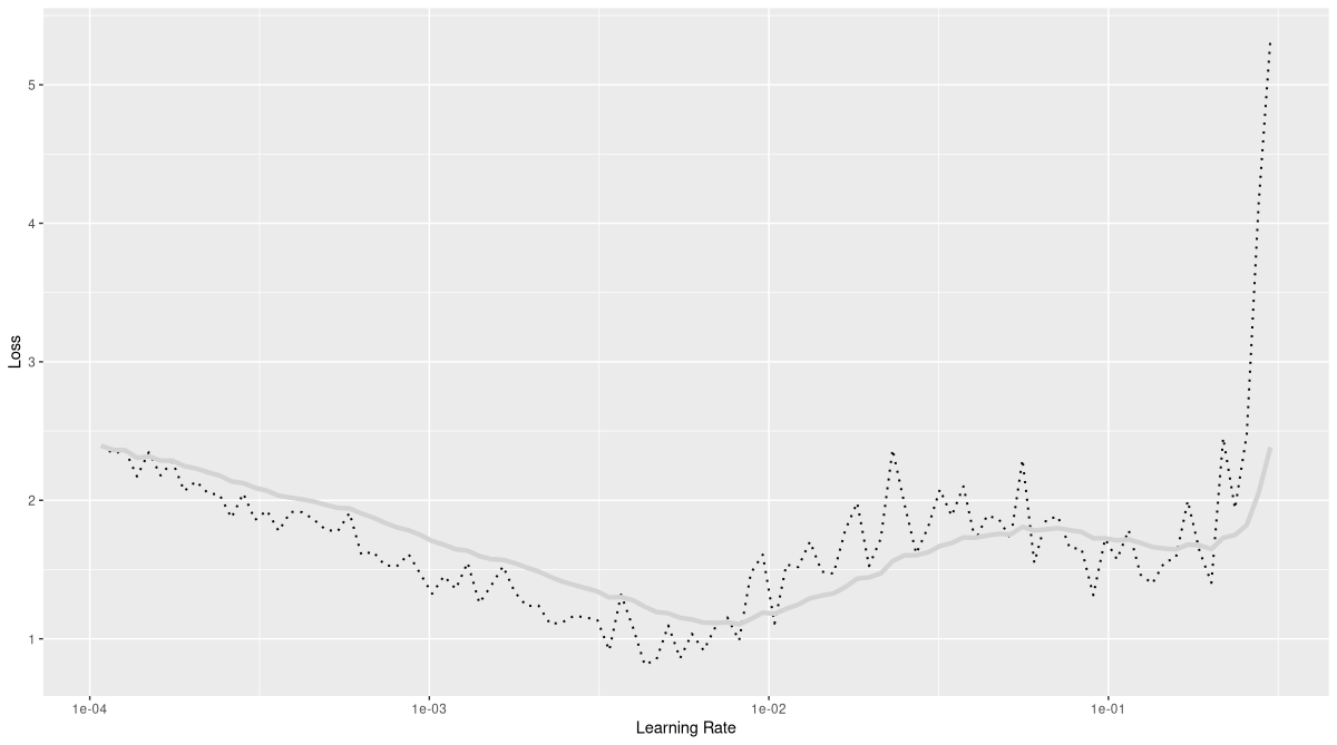
luz’s learning rate finder, run on MNIST.Here, we see that when rates exceed a value of about 0.01, losses become noisy, and increase. The definitive explosion, though, seems to be triggered only when the rate surpasses 0.1. In consequence, you might decide to not exactly follow the “one order of magnitude” recommendation, and try a learning rate of 0.01 – at least in case you do what I’ll be doing in the next section, namely, use the so-determined rate not as a fixed-in-time value, but as a maximal one.
17.2.2 Learning rate schedulers
Once we have an idea where to upper-bound the learning rate, we can make use of one of torch’s learning rate schedulers to orchestrate rates over training. We will decide on a scheduler object, and pass that to a dedicated luz callback: callback_lr_scheduler().
Classically, a popular, intuitively appealing scheme used to be the following. In early stages of training, try a reasonably high learning rate, in order to make quick progress; once that has happened, though, slow down, making sure you don’t zig-zag around (and away from) a presumably-found local minimum.
In the meantime, more sophisticated schemes have been developed.
One family of ideas keeps periodically turning up and down the learning rate. Members of this family are known as, for example, “cyclical learning rates” (Smith (2015)), or (some form of) “annealing with restarts” (e.g., Loshchilov and Hutter (2016)). What differs between members of the family is the shape of the resulting learning rate curve, and the frequency of restarts (meaning, how often you turn up the rate again, to begin a new period of descent). In torch, popular representatives of this family are, for example, lr_cyclic() and lr_cosine_annealing_warm_restarts().
A very different approach is represented by the one-cycle learning rate strategy (Smith and Topin (2017)). In this scheme, we start from some initial – low-ish – learning rate, increase that up to some user-specified maximum, and from there, decrease again, until we’ve arrived at a rate significantly lower than the one we started with. In torch, this is available as lr_one_cycle(), and this is the strategy I was referring to above.
lr_one_cycle() allows for user-side tweaking in a number of ways, and in real-life projects, you may want to play around a bit with its many parameters. Here, we use the defaults. All we need to do, then, is pass in the maximum rate we determined, and decide on how often we want the learning rate to be updated. The logical way seems to be to do it once per batch, something that will happen if we pass in number of epochs and number of steps per epoch.
In the code snippet below, note that the arguments max_lr , epochs, and steps_per_epoch really “belong to” lr_one_cycle(). We have to pass them to the callback, though, because it is the callback that will instantiate the scheduler.
call_on, however, genuinely forms part of the callback logic. This is a harmless-looking argument that, nevertheless, we need to pay attention to. Schedulers differ in whether their period is defined in epochs, or in batches. lr_one_cycle() “wakes up” once per batch; but there are others – lr_step(), for example - that check whether an update is due once per epoch only. The default value of call_on is on_epoch_end; so for lr_one_cycle(), we have to override the default.
num_epochs <- 5

# the model has already been setup(), we continue from there
fitted <- model %>%
  fit(train_dl,
    epochs = num_epochs,
    valid_data = valid_dl,
    callbacks = list(
      luz_callback_lr_scheduler(
        lr_one_cycle,
        max_lr = 0.01,
        epochs = num_epochs,
        steps_per_epoch = length(train_dl),
        call_on = "on_batch_end"
      )
    )
  )
At this point, we wrap up the topic of learning rate optimization. As with so many things in deep learning, research progresses at a rapid rate, and most likely, new scheduling strategies will continue to be added. Now though, for a total change in scope.
17.3 Transfer learning
Transfer, as a general concept, is what happens when we have learned to do one thing, and benefit from those skills in learning something else. For example, we may have learned how to make some move with our left leg; it will then be easier to learn how to do the same with our right leg. Or, we may have studied Latin and then, found that it helped us a lot in learning French. These, of course, are straightforward examples; analogies between domains and skills can be a lot more subtle.
In comparison, the typical usage of “transfer learning” in deep learning seems rather narrow, at first glance. Concretely, it refers to making use of huge, highly effective models (often provided as part of some library), that have already been trained, for a long time, on a huge dataset. Typically, you would load the model, remove its output layer, and add on a small-ish sequential module that takes the model’s now-last layer to the kind of output you require. Often, in example tasks, this will go from the broad to the narrow – as in the below example, where we use a model trained on one thousand categories of images to distinguish between ten types of digits.
But it doesn’t have to be like that. In deep learning, too, models trained on one task can be built upon in tasks that have different, but not necessarily more domain-constrained, requirements. As of today, popular examples for this are found mostly in natural language processing (NLP), a topic we don’t cover in this book. There, you find models trained to predict how a sentence continues – resulting in general “knowledge” about a language – used in logically dependent tasks like translation, question answering, or text summarization. Transfer learning, in that general sense, is something we’ll certainly see more and more of in the near future.
There is another, very important aspect to the popularity of transfer learning, though. When you build on a pre-trained model, you’ll incorporate all of what it has learned - including its biases and preconceptions. How much that matters, in your context, will depend on what exactly you’re doing. For us, who are classifying digits, it will not matter whether the pre-trained model performs a lot better on cats and dogs than on e-scooters, smart fridges, or garbage cans. But think about this whenever models concern people. Typically, these high-performing models have been trained either on benchmark datasets, or data massively scraped from the web. The former have, historically, been very little concerned with questions of stereotypes and representation. (Hopefully, that will change in the future.) The latter are, by definition, subject to availability bias, as well as idiosyncratic decisions made by the dataset creators. (Hopefully, these circumstances and decisions will have been carefully documented. That is something you’ll need to check out.)
With our running example, we’ll be in the former category: We’ll be downstream users of a benchmark dataset. The benchmark dataset in question is ImageNet, the well-known collection of images we already encountered in our first experience with Tiny Imagenet, two chapters ago.
In torchvision, we find a number of ready-to-use models that have been trained on ImageNet. Among them is ResNet-18 (He et al. (2015)). The “Res” in ResNet stands for “residual”, or “residual connection”. Here residual is used, as is common in statistics, to designate an error term. The idea is to have some layers predict, not something entirely new, but the difference between a target and the previous layer’s prediction – the error, so to say. If this sounds confusing, don’t worry. For us, what matters is that due to their architecture, ResNets can afford to be very deep, without becoming excessively hard to train. And that in turn means they’re very performant, and often used as pre-trained feature detectors.
The first time you use a pre-trained model, its weights are downloaded, and cached in an operating-system-specific location.
resnet <- model_resnet18(pretrained = TRUE)
resnet
An `nn_module` containing 11,689,512 parameters.
── Modules ───────────────────────────────────────
• conv1: <nn_conv2d> #9,408 parameters
• bn1: <nn_batch_norm2d> #128 parameters
• relu: <nn_relu> #0 parameters
• maxpool: <nn_max_pool2d> #0 parameters
• layer1: <nn_sequential> #147,968 parameters
• layer2: <nn_sequential> #525,568 parameters
• layer3: <nn_sequential> #2,099,712 parameters
• layer4: <nn_sequential> #8,393,728 parameters
• avgpool: <nn_adaptive_avg_pool2d> #0 parameters
• fc: <nn_linear> #513,000 parametersHave a look at the last module, a linear layer:
resnet$fcFrom the weights, we can see that this layer maps tensors with 512 features to ones with 1000 - the thousand different image categories used in the ImageNet challenge. To adapt this model to our purposes, we simply replace the very last layer with one that outputs feature vectors of length ten:
resnet$fc <- nn_linear(resnet$fc$in_features, 10)
resnet$fc
An `nn_module` containing 5,130 parameters.
── Parameters ───────────────────────────────────────────────────────────────────────────────────────────────
• weight: Float [1:10, 1:512]
• bias: Float [1:10]What will happen if we now train the modified model on MNIST? Training will progress with the speed of a Zenonian tortoise, since gradients need to be propagated across a huge network. Not only is that a waste of time; it is useless, as well. It could, if we were very patient, even be harmful: We could destroy the intricate feature hierarchy learned by the pre-trained model. Of course, in classifying digits we will make use of just a tiny subset of learned higher-order features, but that is not a problem. In any case, with the resources available to mere mortals, we are unlikely to improve on ResNet’s digit-discerning capabilities.
What we do, thus, is set all layer weights to non-trainable, apart from just that last layer we replaced.
Putting it all together, we arrive at the following, concise definition of a model:
convnet <- nn_module(
  initialize = function() {
    self$model <- model_resnet18(pretrained = TRUE)
    for (par in self$parameters) {
      par$requires_grad_(FALSE)
    }
    self$model$fc <- nn_linear(self$model$fc$in_features, 10)
  },
  forward = function(x) {
    self$model(x)
  }
)
This we can now train with luz, like before. There’s just one further step required, and that’s just because I’m using MNIST to illustrate. Since ResNet has been trained on RGB images, its first layer expects three channels, not one. We can work around this by multiplexing the single grayscale channel into three identical ones, using torch_expand(). For important real-life tasks, this may not be an optimal solution; but it will do well enough for MNIST.
A convenient place to perform the expansion is as part of the data pre-processing pipeline, repeated here in modified form.
train_ds <- mnist_dataset(
  dir,
  download = TRUE,
  transform = . %>%
    transform_to_tensor() %>%
    (function(x) x$expand(c(3, 28, 28))) %>%
    transform_random_affine(
      degrees = c(-45, 45), translate = c(0.1, 0.1)
    )
)

train_dl <- dataloader(
  train_ds,
  batch_size = 128,
  shuffle = TRUE
)

valid_ds <- mnist_dataset(
  dir,
  train = FALSE,
  transform = . %>%
    transform_to_tensor %>%
    (function(x) x$expand(c(3, 28, 28)))
)

valid_dl <- dataloader(valid_ds, batch_size = 128)
The code for training then looks as usual.
model <- convnet %>%
  setup(
    loss = nn_cross_entropy_loss(),
    optimizer = optim_adam,
    metrics = list(luz_metric_accuracy())
    ) %>%
  fit(train_dl,
      epochs = 5,
      valid_data = valid_dl)
Before we wrap up both section and chapter, one additional comment. The way we proceeded, above – replacing the very last layer with a single module outputting the final scores – is just the easiest, most straightforward thing to do.
For MNIST, this is good enough. Maybe, on inspection, we’d find that single digits already form part of ResNet’s feature hierarchy; but even if not, a linear layer with ~ 5000 parameters should suffice to learn them. However, the more there is “still to be learned” – equivalently, the more either dataset or task differ from what was used (done, resp.) in model pre-training – the more powerful a sub-module we will want to chain on. We’ll see an example of this in the next chapter.