library(torch)

t1 <- torch_tensor(1)
t13 Tensors
3.1 What’s in a tensor?
To do anything useful with torch, you need to know about tensors. Not tensors in the math/physics sense. In deep learning frameworks such as TensorFlow and (Py-)Torch, tensors are “just” multi-dimensional arrays optimized for fast computation – not on the CPU only but also, on specialized devices such as GPUs and TPUs.
In fact, a torch tensor is like an R array, in that it can be of arbitrary dimensionality. But unlike array, it is designed for fast and scalable execution of mathematical calculations, and you can move it to the GPU. (It also has an extra capability of enormous practical impact – automatic differentiation – but we reserve that for the next chapter.)
Technically, a tensor feels a lot like an R6 object, in that you can access its fields and methods using $-syntax. Let’s create one and print it:
torch_tensor
 1
[ CPUFloatType{1} ]
This is a tensor that holds just a single value, 1. It “lives” on the CPU, and its type is Float . Now take a look at the 1 in braces, {1}. This is not yet another indication of the tensor’s value. It indicates the tensor shape, or put differently: the space it lives in and the extent of its dimensions. Here, we have a one-dimensional tensor, that is, a vector. Just as in base R, vectors can consist of a single element only. (Remember that base R does not differentiate between 1 and c(1)).
We can use the aforementioned $-syntax to individually ascertain these properties, accessing the respective fields in the object one-by-one:
t1$dtypetorch_Floatt1$devicetorch_device(type='cpu')t1$shape[1] 1We can also directly change some of these properties, making use of the tensor object’s $to() method:
t2 <- t1$to(dtype = torch_int())
t2$dtypetorch_Int# only applicable if you have a GPU
t2 <- t1$to(device = "cuda")
t2$devicetorch_device(type='cuda', index=0)How about changing the shape? This is a topic deserving of treatment of its own, but as a first warm-up, let’s play around a bit. Without changing its value, we can turn this one-dimensional “vector tensor” into a two-dimensional “matrix tensor”:
t3 <- t1$view(c(1, 1))
t3$shape
[1] 1 1Conceptually, this is analogous to how in R, we can have a one-element vector as well as a one-element matrix:
c(1)
matrix(1)
[1] 1
[,1]
[1,] 1Now that we have an idea what a tensor is, let’s think about ways to create some.
3.2 Creating tensors
We’ve already seen one way to create a tensor: calling torch_tensor() and passing in an R value. This way generalizes to multi-dimensional objects; we’ll see a few examples soon.
However, that procedure can get unwieldy when we have to pass in lots of different values. Luckily, there is an alternative approach that applies whenever values should be identical throughout, or follow an apparent pattern. We’ll illustrate this technique as well in this section.
3.2.1 Tensors from values
Above, we passed in a one-element vector to torch_tensor(); we can pass in longer vectors just the same way:
torch_tensor(1:5)torch_tensor
1
2
3
4
5
[ CPULongType{5} ]When given an R value (or a sequence of values), torch determines a suitable data type itself. Here, the assumption is that an integer type is desired, and torch chooses the highest-precision type available (torch_long() is synonymous to torch_int64()).
If we want a floating-point tensor instead, we can use $to() on the newly created instance (as we saw above). Alternatively, we can just let torch_tensor() know right away:
torch_tensor(1:5, dtype = torch_float())torch_tensor
1
2
3
4
5
[ CPUFloatType{5} ]Analogously, the default device is the CPU; but we can also create a tensor that, right from the outset, is located on the GPU:
torch_tensor(1:5, device = "cuda")torch_tensor
1
2
3
4
5
[ CPUFloatType{5} ]Now, so far all we’ve been creating is vectors; what about matrices, that is, two-dimensional tensors?
We can pass in an R matrix just the same way:
torch_tensor(matrix(1:9, ncol = 3))torch_tensor
1 4 7
2 5 8
3 6 9
[ CPULongType{3,3} ]Look at the result. The numbers 1 to 9 appear column after column, just as in the R matrix we created it from. This may, or may not, be the intended outcome. If it’s not, just pass byrow = TRUE to the call to matrix():
torch_tensor(matrix(1:9, ncol = 3, byrow = TRUE))torch_tensor
1 2 3
4 5 6
7 8 9
[ CPULongType{3,3} ]What about higher-dimensional data? Following the same principle, we can pass in an array:
torch_tensor(array(1:24, dim = c(4, 3, 2)))torch_tensor
(1,.,.) =
1 13
5 17
9 21
(2,.,.) =
2 14
6 18
10 22
(3,.,.) =
3 15
7 19
11 23
(4,.,.) =
4 16
8 20
12 24
[ CPULongType{4,3,2} ]Again, the result follows R’s array population logic. If that’s not what you want, it is probably easier to build up the tensor programmatically.
Before you start to panic, though, think about how rarely you’ll need to do this. In practice, you’ll mostly be creating tensors from an R dataset. We’ll take a close look at that in the last subsection, “Tensors from datasets”. Before though, it is instructive to spend a little time inspecting that last output.
Here, pictorially, is the object we created (fig. 3.1). Let’s call the axis that extends to the right x, the one that goes into the page, y, and the one that points up, z. Then the tensor extends 4, 3, and 2 units, respectively, in the x, y, and z directions.
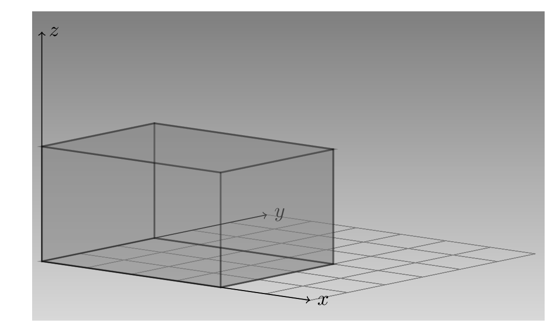
The array we passed to torch_tensor() prints like this:
array(1:24, dim = c(4, 3, 2)), , 1
[,1] [,2] [,3]
[1,] 1 5 9
[2,] 2 6 10
[3,] 3 7 11
[4,] 4 8 12
, , 2
[,1] [,2] [,3]
[1,] 13 17 21
[2,] 14 18 22
[3,] 15 19 23
[4,] 16 20 24Compare that with how the tensor prints, above. Array and tensor slice the object in different ways. The tensor slices its values into 3x2 rectangles, extending up and to the back, one for each of the four x-values. The array, on the other hand, splits them up by z-value, resulting in two big 4x3 slices that go up and to the right.
Alternatively, we could say that the tensor starts thinking from the left/the “outside”; the array, from the right/the “inside”.
3.2.2 Tensors from specifications
There are two broad conditions when torch’s bulk creation functions will come in handy: For one, when you don’t care about individual tensor values, but only about their distribution. Secondly, if they follow some conventional pattern.
When we use bulk creation functions, instead of individual values we specify the shape they should have. Here, for example, we instantiate a 3x3 tensor, populated with standard-normally distributed values:
torch_randn(3, 3)torch_tensor
-0.6532 0.6557 2.0251
-0.7914 -1.7220 1.0387
0.1931 1.0536 -0.2077
[ CPUFloatType{3,3} ]And here is the equivalent for values that are uniformly distributed between zero and one:
torch_rand(3, 3)torch_tensor
0.2498 0.5356 0.6515
0.3556 0.5799 0.1284
0.9884 0.4361 0.8040
[ CPUFloatType{3,3} ]Often, we require tensors of all ones, or all zeroes:
torch_zeros(2, 5)torch_tensor
0 0 0 0 0
0 0 0 0 0
[ CPUFloatType{2,5} ]torch_ones(2, 2)torch_tensor
1 1
1 1
[ CPUFloatType{2,2} ]Many more of these bulk creation functions exist. To wrap up, let’s see how to create some matrix types that are common in linear algebra. Here’s an identity matrix:
torch_eye(n = 5)torch_tensor
1 0 0 0 0
0 1 0 0 0
0 0 1 0 0
0 0 0 1 0
0 0 0 0 1
[ CPUFloatType{5,5} ]And here, a diagonal matrix:
torch_diag(c(1, 2, 3))torch_tensor
1 0 0
0 2 0
0 0 3
[ CPUFloatType{3,3} ]3.2.3 Tensors from datasets
Now we look at how to create tensors from R datasets. Depending on the dataset itself, this process can feel “automatic” or require some thought and action.
First, let’s try JohnsonJohnson that comes with base R. It is a time series of quarterly earnings per Johnson & Johnson share.
JohnsonJohnson Qtr1 Qtr2 Qtr3 Qtr4
1960 0.71 0.63 0.85 0.44
1961 0.61 0.69 0.92 0.55
1962 0.72 0.77 0.92 0.60
1963 0.83 0.80 1.00 0.77
1964 0.92 1.00 1.24 1.00
1965 1.16 1.30 1.45 1.25
1966 1.26 1.38 1.86 1.56
1967 1.53 1.59 1.83 1.86
1968 1.53 2.07 2.34 2.25
1969 2.16 2.43 2.70 2.25
1970 2.79 3.42 3.69 3.60
1971 3.60 4.32 4.32 4.05
1972 4.86 5.04 5.04 4.41
1973 5.58 5.85 6.57 5.31
1974 6.03 6.39 6.93 5.85
1975 6.93 7.74 7.83 6.12
1976 7.74 8.91 8.28 6.84
1977 9.54 10.26 9.54 8.73
1978 11.88 12.06 12.15 8.91
1979 14.04 12.96 14.85 9.99
1980 16.20 14.67 16.02 11.61Can we just pass this to torch_tensor() and magically get what we want?
torch_tensor(JohnsonJohnson)torch_tensor
0.7100
0.6300
0.8500
0.4400
0.6100
0.6900
0.9200
0.5500
0.7200
0.7700
0.9200
0.6000
0.8300
0.8000
1.0000
0.7700
0.9200
1.0000
1.2400
1.0000
1.1600
1.3000
1.4500
1.2500
1.2600
1.3800
1.8600
1.5600
1.5300
1.5900
... [the output was truncated (use n=-1 to disable)]
[ CPUFloatType{84} ]Looks like we can! The values are arranged exactly the way we want them; quarter after quarter.
Magic? Not really. torch can only work with what it is given; and here, what it is given is actually a vector of doubles arranged in quarterly order. The data just print the way they do because they are of class ts:
unclass(JohnsonJohnson)[1] 0.71 0.63 0.85 0.44 0.61 0.69 0.92 0.55 0.72
[10] 0.77 0.92 0.60 0.83 0.80 1.00 0.77 0.92 1.00
[19] 1.24 1.00 1.16 1.30 1.45 1.25 1.26 1.38 1.86
[28] 1.56 1.53 1.59 1.83 1.86 1.53 2.07 2.34 2.25
[37] 2.16 2.43 2.70 2.25 2.79 3.42 3.69 3.60 3.60
[46] 4.32 4.32 4.05 4.86 5.04 5.04 4.41 5.58 5.85
[55] 6.57 5.31 6.03 6.39 6.93 5.85 6.93 7.74 7.83
[64] 6.12 7.74 8.91 8.28 6.84 9.54 10.26 9.54 8.73
[73] 11.88 12.06 12.15 8.91 14.04 12.96 14.85 9.99 16.20
[82] 14.67 16.02 11.61
attr(,"tsp")
[1] 1960.00 1980.75 4.00So this went well. Let’s try another one. Who is not kept up at night, pondering trunk thickness of orange trees?
library(dplyr)

glimpse(Orange)
Rows: 35
Columns: 3
$ Tree <ord> 1, 1, 1, 1, 1, 1, 1, 2, 2, 2, 2, 2, 2,...
$ age <dbl> 118, 484, 664, 1004, 1231, 1372, 1582,...
$ circumference <dbl> 30, 58, 87, 115, 120, 142, 145, 33, 69,...torch_tensor(Orange)Error in torch_tensor_cpp(data, dtype, device, requires_grad,
pin_memory) : R type not handledWhich type is not handled here? It seems obvious that the “culprit” must be Tree, an ordered-factor column. Let’s first check if torch can handle factors:
f <- factor(c("a", "b", "c"), ordered = TRUE)
torch_tensor(f)
torch_tensor
1
2
3
[ CPULongType{3} ]So this worked fine. Then what else could it be? The problem here is the containing structure, the data.frame. We need to call as.matrix() on it first. Due to the presence of the factor, though, this will result in a matrix of all strings, which is not what we want. Therefore, we first extract the underlying levels (integers) from the factor, and then convert the data.frame to a matrix:
orange_ <- Orange %>%
  mutate(Tree = as.numeric(Tree)) %>%
  as.matrix()

torch_tensor(orange_) %>% print(n = 7)
torch_tensor
2 118 30
2 484 58
2 664 87
2 1004 115
2 1231 120
2 1372 142
2 1582 145
... [the output was truncated (use n=-1 to disable)]
[ CPUFloatType{35,3} ]Let’s try the same thing with another data.frame, okc from modeldata:
library(modeldata)

data(okc)
okc %>% glimpse()
Rows: 59,855
Columns: 6
$ age <int> 22, 35, 38, 23, 29, 29, 32, 31, 24,...
$ diet <chr> "strictly anything", "mostly other",...
$ height <int> 75, 70, 68, 71, 66, 67, 65, 65, 67, 65,...
$ location <chr> "south san francisco", "oakland",...
$ date <date> 2012-06-28, 2012-06-29, 2012-06-27,...
$ Class <fct> other, other, other, other, other, stem,...We have two integer columns, which is fine, and one factor column, which we know how to handle. But what about the character and date columns? Trying to create a tensor from the date column individually, we see:
print(torch_tensor(okc$date), n = 7)torch_tensor
15519
15520
15518
15519
15518
15520
15516
... [the output was truncated (use n=-1 to disable)]
[ CPUFloatType{59855} ]This didn’t throw an error, but what does it mean? These are the actual values stored in an R Date, namely, the number of days since January 1, 1970. Technically, thus, we have a working conversion – whether the result makes sense pragmatically is a question of how you’re going to use it. Put differently, you’ll probably want to further process these data before using them in a computation, and how you do this will depend on the context.
Next, let’s see about location, one of the columns of type character. What happens if we just pass it to torch as-is?
torch_tensor(okc$location)Error in torch_tensor_cpp(data, dtype, device, requires_grad,
pin_memory) : R type not handledIn fact, there are no tensors in torch that store strings. We have to apply some scheme that converts them to a numeric type first. In cases like the present one, where every observation contains a single entity (as opposed to, say, a sentence or a paragraph), the easiest way of doing this from R is to first convert to factor, then to numeric, and then, to tensor:
okc$location %>%
  factor() %>%
  as.numeric() %>%
  torch_tensor() %>%
  print(n = 7)
torch_tensor
120
74
102
10
102
102
102
... [the output was truncated (use n=-1 to disable)]
[ CPUFloatType{59855} ]True, this works well technically. It does, however, reduce information. For example, the first and third locations are “south san francisco” and “san francisco”, respectively. Once converted to factors, these are just as distant, semantically, as are “san francisco” and any other location. Again, whether this is of relevance depends on the specifics of the data, as well as your goal. If you think it does matter, you have a range of options, including, for example, grouping observations by some criterion, or converting to latitude/longitude. These considerations are by no means torch-specific; we just mention them here because they affect the “data ingestion workflow” to torch.
Finally, no excursion into the world of real-life data science is complete without a consideration of NAs. Let’s see:
torch_tensor(c(1, NA, 3))torch_tensor
1
nan
3
[ CPUFloatType{3} ]R’s NA gets converted to NaN. Can you work with that? Some torch function can. For example, torch_nanquantile() just ignores the NaNs:
torch_nanquantile(torch_tensor(c(1, NA, 3)), q = 0.5)torch_tensor
2
[ CPUFloatType{1} ]However, if you’re going to train a neural network, for example, you’ll need to think about how to meaningfully replace these missing values first. But that’s a topic for a later time.
3.3 Operations on tensors
We can perform all the usual mathematical operations on tensors.: add, subtract, divide … These operations are available as functions (starting with torch_) as well as as methods on objects (invoked with $-syntax). For example, the following are equivalent:
t1 <- torch_tensor(c(1, 2))
t2 <- torch_tensor(c(3, 4))

torch_add(t1, t2)
# equivalently
t1$add(t2)
torch_tensor
4
6
[ CPUFloatType{2} ]In both cases, a new object is created; neither t1 nor t2 are modified. There exists an alternate method that modifies its object in-place:
t1$add_(t2)torch_tensor
4
6
[ CPUFloatType{2} ]t1torch_tensor
4
6
[ CPUFloatType{2} ]In fact, the same pattern applies for other operations: Whenever you see an underscore appended, the object is modified in-place.
Naturally, in a scientific-computing setting, matrix operations are of special interest. Let’s start with the dot product of two one-dimensional structures, i.e., vectors.
t1 <- torch_tensor(1:3)
t2 <- torch_tensor(4:6)
t1$dot(t2)
torch_tensor
32
[ CPULongType{} ]Were you thinking this shouldn’t work? Should we have needed to transpose (torch_t()) one of the tensors? In fact, this also works:
t1$t()$dot(t2)torch_tensor
32
[ CPULongType{} ]The reason the first call worked, too, is that torch does not distinguish between row vectors and column vectors. In consequence, if we multiply a vector with a matrix, using torch_matmul(), we don’t need to worry about the vector’s orientation either:
t3 <- torch_tensor(matrix(1:12, ncol = 3, byrow = TRUE))
t3$matmul(t1)
torch_tensor
14
32
50
68
[ CPULongType{4} ]The same function, torch_matmul(), would be used to multiply two matrices. Note how this is different from what torch_multiply() does, namely, scalar-multiply its arguments:
torch_multiply(t1, t2)torch_tensor
4
10
18
[ CPULongType{3} ]Many more tensor operations exist, some of which you’ll meet over the course of this journey. But there is one group that deserves special mention.
3.3.1 Summary operations
If you have an R matrix and are about to compute a sum, this could, normally, mean one of three things: the global sum, row sums, or column sums. Let’s see all three of them at work (using apply() for a reason):
m <- outer(1:3, 1:6)

sum(m)
apply(m, 1, sum)
apply(m, 2, sum)
[1] 126
[1] 21 42 63
[1] 6 12 18 24 30 36And now, the torch equivalents. We start with the overall sum.
t <- torch_outer(torch_tensor(1:3), torch_tensor(1:6))
t$sum()
torch_tensor
126
[ CPULongType{} ]It gets more interesting for the row and column sums. The dim argument tells torch which dimension(s) to sum over. Passing in dim = 1, we see:
t$sum(dim = 1)torch_tensor
6
12
18
24
30
36
[ CPULongType{6} ]Unexpectedly, these are the column sums! Before drawing conclusions, let’s check what happens with dim = 2:
t$sum(dim = 2)torch_tensor
21
42
63
[ CPULongType{3} ]Now, we have sums over rows. Did we misunderstand something about how torch orders dimensions? No, it’s not that. In torch, when we’re in two dimensions, we think rows first, columns second. (And as you’ll see in a minute, we start indexing with 1, just as in R in general.)
Instead, the conceptual difference is specific to aggregating, or “grouping”, operations. In R, grouping, in fact, nicely characterizes what we have in mind: We group by row (dimension 1) for row summaries, by column (dimension 2) for column summaries. In torch, the thinking is different: We collapse the columns (dimension 2) to compute row summaries, the rows (dimension 1) for column summaries.
The same thinking applies in higher dimensions. Assume, for example, that we been recording time series data for four individuals. There are two features, and both of them have been measured at three times. If we were planning to train a recurrent neural network (much more on that later), we would arrange the measurements like so:
Dimension 1: Runs over individuals.
Dimension 2: Runs over points in time.
Dimension 3: Runs over features.
The tensor then would look like this:
t <- torch_randn(4, 3, 2)
t
torch_tensor
(1,.,.) =
-1.3427 1.1303
1.0430 0.8232
0.7952 -0.2447
(2,.,.) =
-1.9929 0.1251
0.4143 0.3523
0.9819 0.3219
(3,.,.) =
0.6389 -0.2606
2.4011 0.2656
-0.1750 -0.2597
(4,.,.) =
1.4534 0.7229
1.2503 -0.2975
1.6749 -1.2154
[ CPUFloatType{4,3,2} ]To obtain feature averages, independently of subject and time, we would collapse dimensions 1 and 2:
t$mean(dim = c(1, 2))torch_tensor
-0.1600
0.1363
[ CPUFloatType{2} ]If, on the other hand, we wanted feature averages, but individually per person, we’d do:
t$mean(dim = 2)torch_tensor
-0.6153 0.8290
0.3961 0.2739
-0.0579 0.1966
-0.3628 -0.7544
[ CPUFloatType{4,2} ]Here, the single feature “collapsed” is the time step.
3.4 Accessing parts of a tensor
Often, when working with tensors, some computational step is meant to operate on just part of its input tensor. When that part is a single entity (value, row, column …), we commonly refer to this as indexing; when it’s a range of such entities, it is called slicing.
3.4.1 “Think R”
Both indexing and slicing work essentially as in R. There are a few syntactic extensions, and I’ll present these in the subsequent section. But overall you should find the behavior intuitive.
This is because just as in R, indexing in torch is one-based. And just as in R, singleton dimensions are dropped.
In the below example, we ask for the first column of a two-dimensional tensor; the result is one-dimensional, i.e., a vector:
t <- torch_tensor(matrix(1:9, ncol = 3, byrow = TRUE))
t[1, ]
torch_tensor
1
2
3
[ CPULongType{3} ]If we specify drop = FALSE, though, dimensionality is preserved:
t[1, , drop = FALSE]torch_tensor
1 2 3
[ CPULongType{1,3} ]When slicing, there are no singleton dimensions – and thus, no additional considerations to be taken into account:
t <- torch_rand(3, 3, 3)
t[1:2, 2:3, c(1, 3)]
torch_tensor
(1,.,.) =
0.5273 0.3781
0.5303 0.9537
(2,.,.) =
0.2966 0.7160
0.5421 0.4284
[ CPUFloatType{2,2,2} ]In sum, thus, indexing and slicing work very much like in R. Now, let’s look at the aforementioned extensions that further enhance usability.
3.4.1.1 Beyond R
One of these extensions concerns accessing the last element in a tensor. Conveniently, in torch, we can use -1 to accomplish that:
t <- torch_tensor(matrix(1:4, ncol = 2, byrow = TRUE))
t[-1, -1]
torch_tensor
4
[ CPULongType{} ]Note how in R, negative indices have a quite different effect, causing elements at respective positions to be removed.
Another useful feature extends slicing syntax to allow for a step pattern, to be specified after a second colon. Here, we request values from every second column between columns one and eight:
t <- torch_tensor(matrix(1:20, ncol = 10, byrow = TRUE))
t[ , 1:8:2]
torch_tensor
1 3 5 7
11 13 15 17
[ CPULongType{2,4} ]Finally, sometimes the same code should be able to work with tensors of different dimensionalities. In this case, we can use .. to collectively designate any existing dimensions not explicitly referenced.
For example, say we want to index into the first dimension of whatever tensor is passed, be it a matrix, an array, or some higher-dimensional structure. The following
t[1, ..]will work for all:
t1 <- torch_randn(2, 2)
t2 <- torch_randn(2, 2, 2)
t3 <- torch_randn(2, 2, 2, 2)
t1[1, ..]
t2[1, ..]
t3[1, ..]
torch_tensor
-0.6179
-1.4769
[ CPUFloatType{2} ]
torch_tensor
1.0602 -0.9028
0.2942 0.4611
[ CPUFloatType{2,2} ]
torch_tensor
(1,.,.) =
1.3304 -0.6018
0.0825 0.1221
(2,.,.) =
1.7129 1.2932
0.2371 0.9041
[ CPUFloatType{2,2,2} ]If we wanted to index into the last dimension instead, we’d write t[.., 1]. We can even combine both:
t3[1, .., 2]torch_tensor
-0.6018 0.1221
1.2932 0.9041
[ CPUFloatType{2,2} ]Now, a topic just as important as indexing and slicing is reshaping of tensors.
3.5 Reshaping tensors
Say you have a tensor with twenty-four elements. What is its shape? It could be any of the following:
a vector of length 24
a matrix of shape 24 x 1, or 12 x 2, or 6 x 4, or …
a three-dimensional array of size 24 x 1 x 1, or 12 x 2 x 1, or …
and so on (in fact, it could even have shape 24 x 1 x 1 x 1 x 1)
We can modify a tensor’s shape, without juggling around its values, using the view() method. Here is the initial tensor, a vector of length 24:
t <- torch_zeros(24)
print(t, n = 3)
torch_tensor
0
0
0
... [the output was truncated (use n=-1 to disable)]
[ CPUFloatType{24} ]Here is that same vector, reshaped to a wide matrix:
t2 <- t$view(c(2, 12))
t2
torch_tensor
0 0 0 0 0 0 0 0 0 0 0 0
0 0 0 0 0 0 0 0 0 0 0 0
[ CPUFloatType{2,12} ]So we have a new tensor, t2, but interestingly (and importantly, performance-wise), torch did not have to allocate any new storage for its values. This we can verify for ourselves. Both tensors store their data in the same location:
t$storage()$data_ptr()
t2$storage()$data_ptr()
[1] "0x55cd15789180"
[1] "0x55cd15789180"Let’s talk a bit about how this is possible.
3.5.1 Zero-copy reshaping vs. reshaping with copy
Whenever we ask torch to perform an operation that changes the shape of a tensor, it tries to fulfill the request without allocating new storage for the tensor’s contents. This is possible because the same data – the same bytes, ultimately – can be read in different ways. All that is needed is storage for the metadata.
How does torch do it? Let’s see a concrete example. We start with a 3 x 5 matrix.
t <- torch_tensor(matrix(1:15, nrow = 3, byrow = TRUE))
t
torch_tensor
1 2 3 4 5
6 7 8 9 10
11 12 13 14 15
[ CPULongType{3,5} ]Tensors have a stride() method that tracks, for every dimension, how many elements have to be traversed to arrive at its next element. For the above tensor t, to go to the next row, we have to skip over five elements, while to go to the next column, we need to skip just one:
t$stride()[1] 5 1Now we reshape the tensor so it has five rows and three columns instead. Remember, the data themselves do not change.
t2 <- t$view(c(5, 3))
t2
torch_tensor
1 2 3
4 5 6
7 8 9
10 11 12
13 14 15
[ CPULongType{5,3} ]This time, to arrive at the next row, we just skip three elements instead of five. To get to the next column, we still just “jump over” a single element only:
t2$stride()[1] 3 1Now you may be thinking, what if the order of the elements also has to change? For example, in matrix transposition. Is that still doable with the metadata-only approach?
t3 <- t$t()
t3
torch_tensor
1 6 11
2 7 12
3 8 13
4 9 14
5 10 15
[ CPULongType{5,3} ]In fact, it must be, as both the original tensor and its transpose point to the same place in memory:
t$storage()$data_ptr()
t3$storage()$data_ptr()
[1] "0x55cd1cd4a840"
[1] "0x55cd1cd4a840"And it makes sense: This will work if we know that to arrive at the next row, we just skip a single element, while to arrive at the next column, that’s five to skip over now. Let’s verify:
t3$stride()[1] 1 5Exactly.
Whenever possible, torch will try to handle shape-changing operations in this way.
Another such zero-copy operation (and one we’ll see a lot) is squeeze(), together with its antagonist, unsqueeze(). The latter adds a singleton dimension at the requested position, the former removes it. For example:
t <- torch_randn(3)
t

t$unsqueeze(1)
torch_tensor
0.2291
-0.9454
1.6630
[ CPUFloatType{3} ]
torch_tensor
0.2291 -0.9454 1.6630
[ CPUFloatType{1,3} ]Here we added a singleton dimension in front. Alternatively, we could have used t$unsqueeze(2) to add it at the end.
Now, will that zero-copy technique ever fail? Here is an example where it does:
t <- torch_randn(3, 3)
t$t()$view(9)
Error in (function (self, size) :
view size is not compatible with input tensor's size and
stride (at least one dimension spans across two contiguous
subspaces). Use .reshape(...) instead. [...]When two operations that change the stride are executed in sequence, the second is pretty likely to fail. There is a way to exactly determine whether it will fail or not; but the easiest way is to just use a different method instead of view(): reshape(). The latter will “automagically” work metadata-only if that is possible, but make a copy if not:
t <- torch_randn(3, 3)
t2 <- t$t()$reshape(9)

t$storage()$data_ptr()
t2$storage()$data_ptr()
[1] "0x55cd1622a000"
[1] "0x55cd19d31e40"As expected, both tensors are now stored in different locations.
Finally, we are going to end this long chapter with a feature that may seem overwhelming at first, but is of tremendous importance performance-wise. Like with so many things, it takes time to get accustomed to, but rest assured: You’ll encounter it again and again, in this book and in many projects using torch. It is called broadcasting.
3.6 Broadcasting
We often have to perform operations on tensors with shapes that don’t match exactly.
Of course, we wouldn’t probably try to add, say, a length-two vector to a length-five vector. But there are things we may want to do: for example, multiply every element by a scalar. This works:
t1 <- torch_randn(3, 5)
t1 * 0.5
torch_tensor
-0.4845 0.3092 -0.3710 0.3558 -0.2126
-0.3419 0.1160 0.1800 -0.0094 -0.0189
-0.0468 -0.4030 -0.3172 -0.1558 -0.6247
[ CPUFloatType{3,5} ]That was probably a bit underwhelming. We’re used to that; from R. But the following does not work in R. The intention here would be to add the same vector to every row in a matrix:
m <- matrix(1:15, ncol = 5, byrow = TRUE)
m2 <- matrix(1:5, ncol = 5, byrow = TRUE)

m + m2
Error in m + m2 : non-conformable arraysNeither does it help if we make m2 a vector.
m3 <- 1:5

m + m3
[,1] [,2] [,3] [,4] [,5]
[1,] 2 6 5 9 8
[2,] 8 12 11 10 14
[3,] 14 13 17 16 20Syntactically this worked, but semantics-wise this is not what we intended.
Now, we try both of the above with torch. First, again, the scenario where both tensors are two-dimensional (even though, conceptually, one of them is a row vector):
t <- torch_tensor(m)
t2 <- torch_tensor(m2)

t$shape
t2$shape

t$add(t2)
[1] 3 5
[1] 1 5
torch_tensor
  2   4   6   8  10
  7   9  11  13  15
 12  14  16  18  20
[ CPULongType{3,5} ]
And now, with the thing to be added a one-dimensional tensor:
t3 <- torch_tensor(m3)

t3$shape

t$add(t3)
[1] 5
torch_tensor
2 4 6 8 10
7 9 11 13 15
12 14 16 18 20
[ CPULongType{3,5} ]In torch, both ways worked as intended. Let’s see why.
Above, I’ve printed the tensor shapes for a reason. To a tensor of shape 3 x 5, we were able to add both a tensor of shape 3 and a tensor of shape 1 x 5. Together, these illustrate how broadcasting works. In a nutshell, this is what happens:
The 1 x 5 tensor, when used as an addend, is virtually expanded, that is, treated as if it contained the same row three times. This kind of expansion can only be performed if the non-matching dimension is a singleton, and if it is located on the left.
The same thing happens to the shape-3 tensor, but there is one additional step that takes place first: A leading dimension of size 1 is – virtually – appended on the left. This puts us in exactly the same state we were in in (1), and we continue from there.
Importantly, no physical expansions take place.
Let’s systematize these rules.
3.6.1 Broadcasting rules
The rules are the following. The first, unspectactular though it may look, is the basis for everything else.
- We align tensor shapes, starting from the right.
Say we have two tensors, one of size 3 x 7 x 1, the other of size 1 x 5. Here they are, right-aligned:
# t1, shape:        3  7  1
# t2, shape: 1 5- Starting from the right, the sizes along aligned axes either have to match exactly, or one of them has to be equal to 1. In the latter case, the singleton-dimension tensor is broadcast to the non-singleton one.
In the above example, broadcasting happens twice – once for each tensor. This (virtually) yields
# t1, shape:        3  7  5
# t2, shape: 7 5- If, on the left, one of the tensors has an additional axis (or more than one), the other is virtually expanded to have a dimension of size 1 in that place, in which case broadcasting will occur as stated in (2).
In our example, this happens to the second tensor. First, there is a virtual expansion
# t1, shape:        3  7  5
# t2, shape:        1  7  5
and then, broadcasting takes place:
# t1, shape:        3  7  5
# t2, shape:        3  7  5
In this example, we see that broadcasting can act on both tensors at the same time. The thing to keep in mind, though, is that we always start looking from the right. For example, no broadcasting in the world could make this work:
torch_zeros(4, 3, 2, 1)$add(torch_ones(4, 3, 2)) # error!Now, that was one of the longest, and least applied-seeming, perhaps, chapters in the book. But feeling comfortable with tensors is, I dare say, a precondition for being fluent in torch. The same goes for the topic covered in the next chapter, automatic differentiation. But the difference is, there torch does all the heavy lifting for us. We just need to understand what it’s doing.